GCNN: Gated CNN
One of the major defects of Seq2Seq models is that it can’t process words in parallel. For a large corpus of text, this increases the time spent translating the text. CNNs can help us solve this problem. In this paper: “Language Modeling with Gated Convolutional Networks”, proposed by FAIR (Facebook AI Research) in 2017, the researchers developed a new architecture that uses gating mechanism over stacked convolution layers that outperforms the Seq2Seq model.

Using stacked convolutions layers is more efficient since it allows parallelization over sequential tokens. Using a kernel size of $k$ over a context of size $N$, this new architecture will perform $O\left( \frac{N}{k} \right)$ operations unlike recurrent networks which will perform a linear number $O\left( N \right)$ of operations. The former figure illustrates the model architecture; where:
-
The input to the model is a sequence of words $w_{0},\ …w_{N}$.
-
Each word is represented by a vector embedding stored in a lookup table $D^{\left| V \right| \times e}$ where $\left| V \right|$ is the vocabulary and $e$ is the embedding size.
-
After the lookup table, the input will be represented as word embeddings:
- The hidden layers $h_{0},\ …h_{L}$, where $L$ is the number of layers, are computed as:
Where $X \in \mathbb{R}^{N \times m}$ is the input of layer $h_{l}$ (either word embeddings or the outputs of previous layers), $W \in \mathbb{R}^{k \times m \times n}$, $b \in \mathbb{R}^{n}$, $V \in \mathbb{R}^{k \times m \times n}$, and $c \in \mathbb{R}^{n}$ are learned parameters, $m$ and $n$ are respectively the number of input and output feature maps, $\sigma$ is the sigmoid function and $\otimes$ is the element-wise product between matrices.
Note:
When convolving inputs, they made sure that $h_{i}$ does not contain information from future words by shifting the convolutional inputs to prevent the kernels from seeing future context.
Adaptive Softmax
The simplest choice to To obtain model’s predictions at the last layer is to use a softmax layer, but this choice is often computationally inefficient for large vocabularies. A better choice could be hierarchical softmax (Morin & Bengio, 2005).
In the paper, they chose an improvement of the latter known as adaptive softmax which assigns higher capacity to very frequent words and lower capacity to rare words. This results in lower memory requirements as well as faster computation at both training and test time. You can find an efficient implementation of Adaptive Softmax in Facebook Research’s official GitHub repository: facebookresearch/adaptive-softmax.
Experiments
All experiments in this paper were using two public large-scale language modeling datasets: Google’s Billion word dataset (one billion token) and WikiText-103 dataset (100M tokens). For both datasets, $\left\langle S \right\rangle$ and $\left\langle /S \right\rangle$ tokens were added at the start and end of each line respectively. In terms of optimization, they initialized the layers of the model with the He initialization with the learning rate sampled uniformly in the interval $\lbrack 1.,\ 2.\rbrack$, the momentum was set to $0.99$, and gradient clipping was set to $0.1$ to prevent gradient explosion. Also, weight normalization was used to make training faster as seen in the following figure:

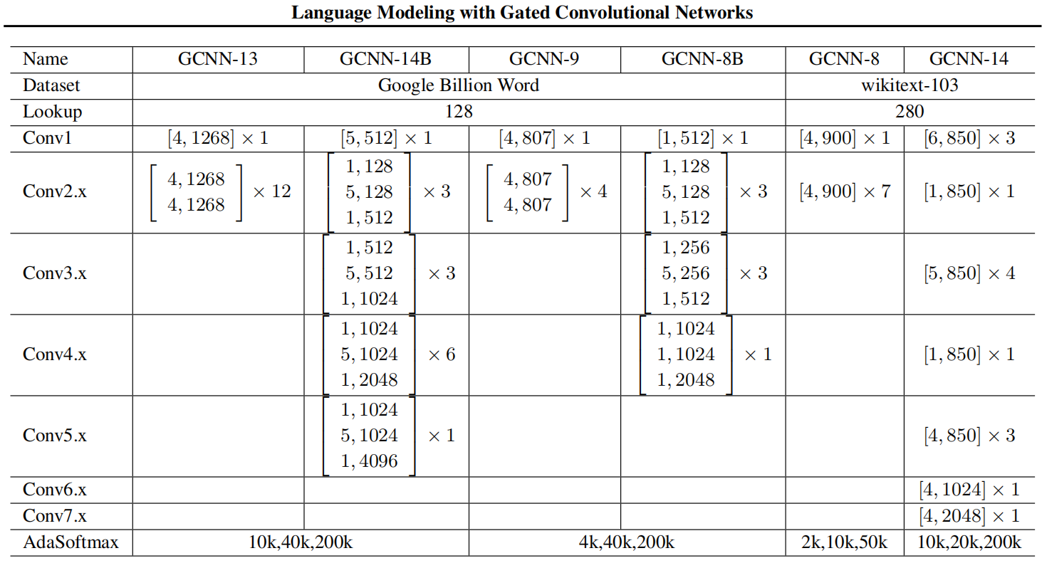
For model architecture, they selected the number of residual blocks between $\left{ 1,\ …10 \right}$, the size of the embeddings with $\left{ 128,\ …256 \right}$, the number of units between $\left{ 128,\ …2048 \right}$, and the kernel width between $\left{ 3,\ …5 \right}$ as shown in the following table:
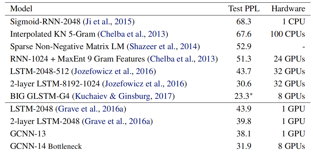
The following table shows the test perplexity over Google’s Billion word dataset; as we can see, GCNN outperforms all LSTMs with the same output approximation while only requiring a fraction of the operations:
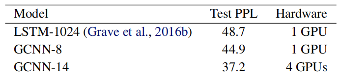
Same thing happens with WikiText-103 dataset; GCNN outperforms LSTM models:
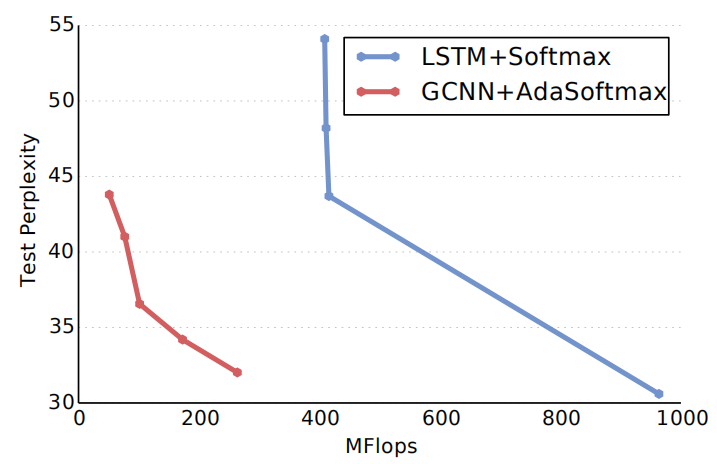
The following figure shows a comparison between GCNN and the state-of-the-art LSTM model back in 2016 which uses the full softmax, the adaptive softmax approximation greatly reduces the number of operations required to reach a given perplexity:
Gating Mechanism (GLU)
Gating mechanisms control the path through which information flows in the network. LSTMs enable long-term memory via a separate cell controlled by different gates (forget, update, output gates). This allows information to flow through potentially many timesteps and without these gates, information could easily vanish.
In contrast, convolutional networks do not suffer from the same kind of vanishing gradient and we find experimentally that they do not require forget gates. Therefore, they considered using only output gates, which allow the network to control what information should be propagated through the hierarchy of layers.
In this paper, they tried four different output gating mechanisms on the WikiText-103 benchmark:
- Tanh (not gating mechanism):
- ReLU (not gating mechanism):
- Gated Tanh Unit (GTU):
- Gated Linear Unit (GLU):
And the results show that GLU achieves the best perplexity over the data as seen in the following figure. There is a gap of about 5 perplexity points between the GLU and ReLU which is similar to the difference between the LSTM and RNN models on the same dataset.

Note:
The difference between GTU and $\text{Tanh}$ models shows us the effect
of gating mechanism since the $\text{Tanh}$ model can be thought of as a
GTU network with the sigmoid gating units removed:
The experiments so far have shown that the GLU benefits from the linear path the unit provides compared to other non-linearities such as GTU. That’s why they decided to compare GLU to purely linear networks in order to measure the impact of the nonlinear path provided by the gates of the GLU. In the paper, they compared GLU to:
- Linear (not gating mechanism):
- Bi-linear:
The following figure shows the performance of the three mechanisms on Google’s Billion word benchmark. As we can see, GLU still outperforms other methods

Context Size $k$
The following figure shows the impact of context size for GCNN on Google’s Billion word dataset (left graph) and WikiText-103 dataset (right graph). Generally, larger contexts improve accuracy but returns drastically diminish with windows larger than 40 words:
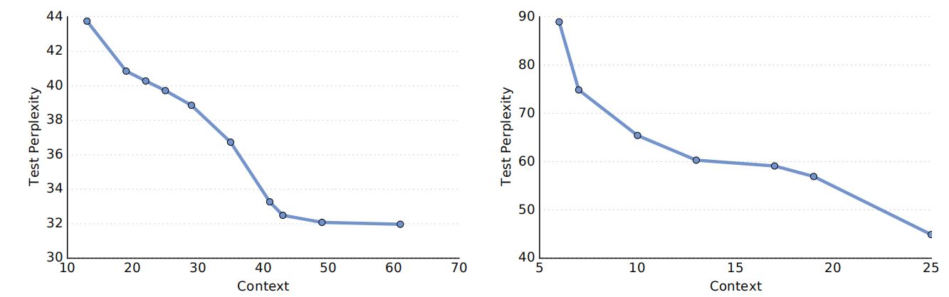
The previous figure Figure 4 also shows that WikiText-103 benefits much more from larger context size than Google Billion Word as the performance degrades more sharply with smaller contexts.