ConvS2S
One of the major defects of Seq2Seq models is that it can’t process words in parallel. For a large corpus of text, this increases the time spent translating the text. CNNs can help us solve this problem. In this paper: “Convolutional Sequence to Sequence Learning”, proposed by FAIR (Facebook AI Research) in 2017. The official repository for this paper can be found on fairseq/convs2s.
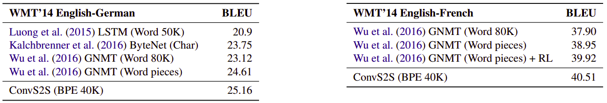
In this paper, we can see that ConvS2S outperformed the Attention model on both WMT’14 English-German and WMT’14 English-French translation using an entirely-CNN translation model with faster results.
The following figure shows the whole ConvS2S architecture created by Facebook AI Research (FAIR):
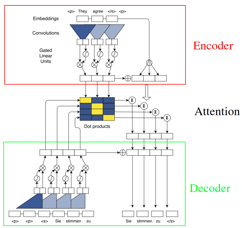
As we can see, this architecture seems a bit complicated and consists of many different components that need clarification. So, let’s divide this big architecture into three main components: Encoder, Decoder and Attention.
Encoder
The encoder component consists of five different steps:
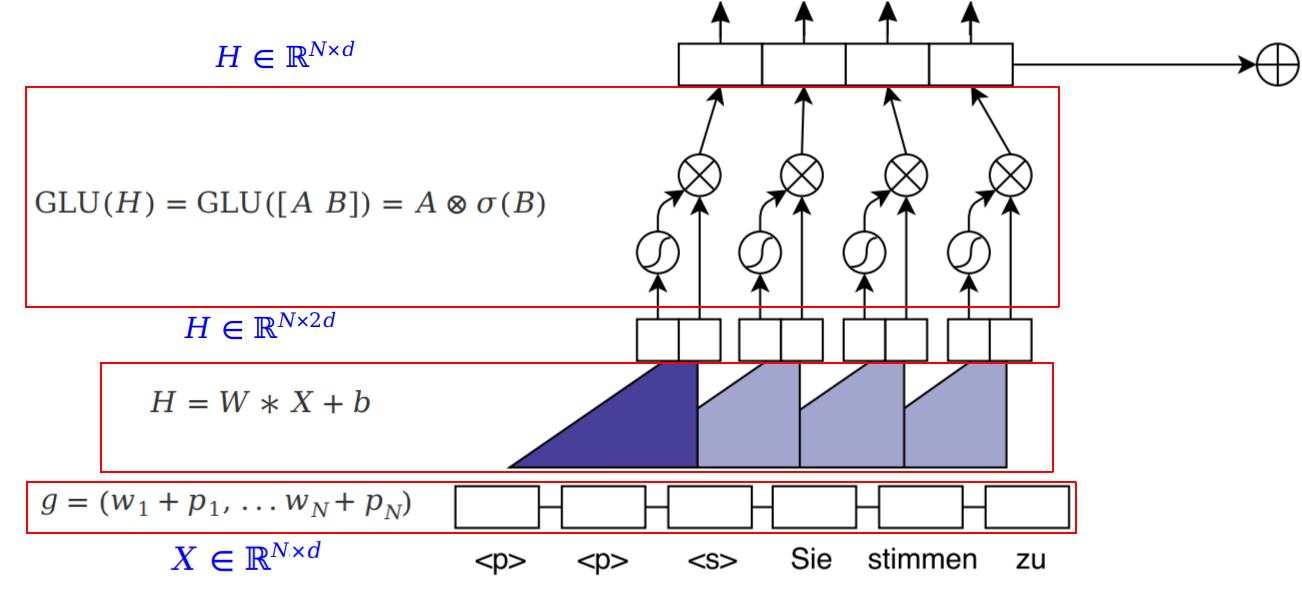
- Padding: The recurrent neural nets process text from left-to-right while in CNNs the words that are close together get convoluted together. So, if we have a sentence of $L$ words and the representative word vector is $d$ features long, then we can represent the sentence as a 2D-plane $X \in \mathbb{R}^{L \times d}$. And to ensure that the output of the convolution layers matches the input length, we apply padding to the input at each layer based on the following formula given that $k$ is the kernel height (the kernel’s width is always the same as the input’s width):
Padding is denoted by the <p> tag which is usually zero as shown in the following image:

- Position Embedding: Then, we use word-embedding $w$ (of size 512 in the paper) combined with the absolute position $p$ of the words to obtain word-position knowing that the size of $p$ is the same as $w$:
- Convolution: Now, we have a matrix representing the input sentence $X \in \mathbb{R}^{L \times d}$ where $L$ is the length of the sentence. Next, we are going to use convolution of $2d$ different filters, each convolution kernel is a $W \in \mathbb{R}^{k \times d}$ where $k$ is the kernel size. Performing the convolution will result into a matrix of $Z \in \mathbb{R}^{L \times 2d}$.
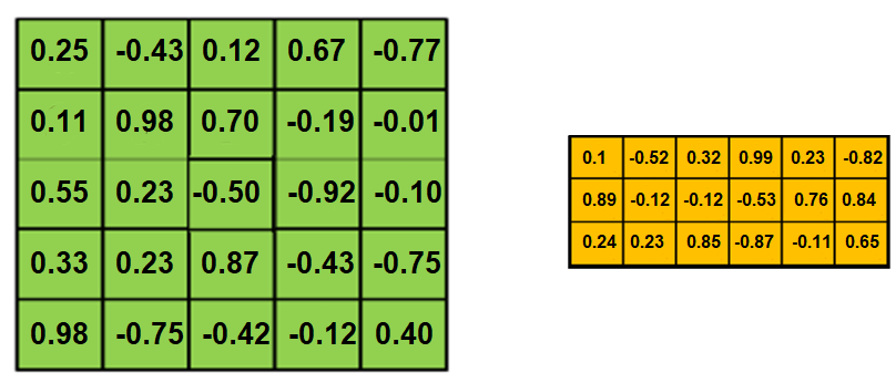
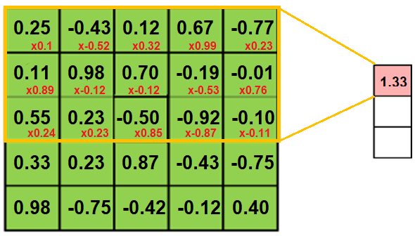
In the following example, we are going to use a $3 \times d$ filters (trigram filters). When we convolve a filter with a sentence, we multiply its values element-wise with the original matrix, then summing them up. We keep doing that till we pass through the whole sentence with a certain number of filters.
- GLU: After applying convolution, we will have an output of $Z \in \mathbb{R}^{L \times 2d}$ over which we are going to apply GLU (Gated-Linear Unit). We are going to split $Z$ into two matrices $A \in \mathbb{R}^{L \times d}$ and $B \in \mathbb{R}^{L \times d}$. Applying GLU means applying the following formula:
Where $\otimes$ is the point-wise multiplication and $\sigma$ is the sigmoid function. The term $\sigma(B)$ controls which inputs $A$ of the current context are relevant.
- Residual: To enable deep layers, we add residual connections from the input of each convolution layer to the output from GLU step.
After applying the residual connection, we multiply the sum of the input and output of a residual block by $\sqrt{0.5}$ to halve the variance of the sum.
Here is the encoder with input dimensions for reference:

Decoder
The decoder is the same as the encoder after removing the **residual part**:
- Padding: Padding in the decoder is a little bit different than the encoding. Here, we pad the input using ($k - 1$) on both sides instead of $\frac{k - 1}{2}$ where $k$ is the kernel height:
- Embedding: The same as the encoder.
- Convolution: The same as the encoder.
- GLU: The same as the encoder.
Here is the decoder with input dimensions for reference:
Now, we have discussed the encoder and the decoder part of the ConvS2S architecture. Let’s get to the attention mechanism which is used in this architecture.
Attention
In the following part, we are going to discuss the attention mechanism used in this architecture. Before getting into this, let’s recap a few terms:
-
The output matrix of the encoder is $Z \in \mathbb{R}^{L \times d}$ where $L$ is the length of the encoder’s input sequence and $d$ is the embedding size.
-
The output matrix of the decoder is $H \in \mathbb{R}^{N \times d}$ where $N$ is the length of the decoder’s input sequence.
-
$e = \left( e_{1},\ …\ e_{L} \right)$ is the element embedding for the encoder sequence. While $g = \left( g_{1},\ …\ g_{N} \right)$ is the element embedding for the decoder sequence.
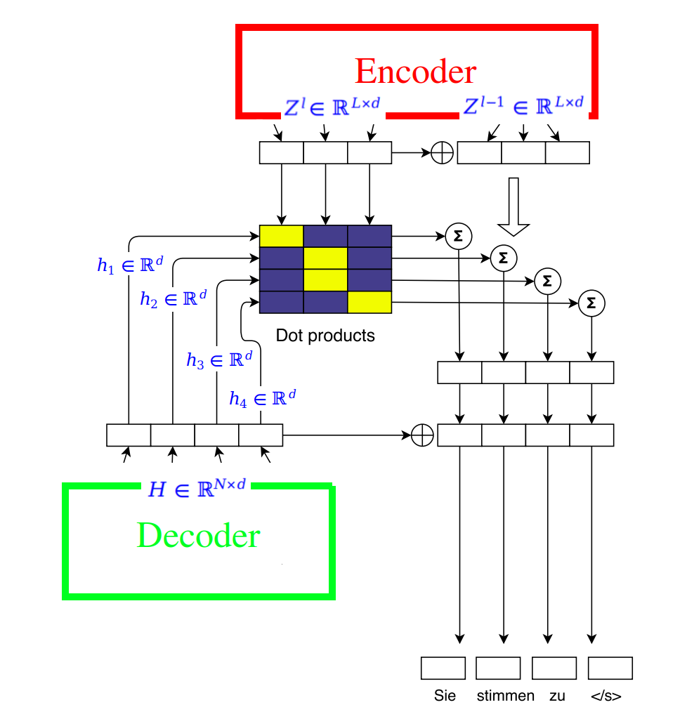
To compute the attention, we follow the following steps:
- First, we combine the the decoder’s current state $h_{i}^{l}$ with the decoder’s embedding embedding $g_{i}$ to get the decoder state summary $d_{i}^{l}$:
- For decoder layer $l$, the attention $a_{\text{ij}}^{l}$ of state $i$ and source element $j$ is computed as a dot-product between the decoder state summary $d_{i}^{l}$ and each output $Z^{u} = \left( z_{1}^{u},\ …\ z_{L}^{u} \right)$ of the last encoder block $u$:
- The conditional input $c_{i}^{l}$ to the current decoder layer is a weighted sum of the encoder outputs $z_{j}^{u}$ as well as the input element embeddings $e_{j}$. The term $L\sqrt{\frac{1}{L}}$ is used to scale up the result.
The attention mechanism can be summarized in the following image:
The problem is that Convolutional Neural Networks do not necessarily help with the problem of figuring out the problem of dependencies when translating sentences. That’s why Transformers were created, they are a combination of both CNNs with attention.
Initialization
The motivation for their initialization is to maintain the variance of activations throughout the forward and backward passes. The following is the different initialization for different parts of the architecture:
-
All embeddings are initialized from a normal distribution $\mathcal{N}\left( 0,\ 0.1 \right)$.
-
For layers whose output is not directly fed to a gated linear unit, they initialized the weights from the normal distribution $\mathcal{N}\left( 0,\ \sqrt{\frac{1}{n_{l}}} \right)$ where $n_{l}$ is the number of input connections to each neuron at layer $l$.
-
For layers which are followed by a GLU activation, they initialized the weights from the normal distribution $\mathcal{N}\left( 0,\ \sqrt{\frac{4}{n_{l}}} \right)$.
-
They applied dropout to the input of some layers so that inputs are retained with a probability of $p$.
-
Biases are uniformly set to zero when the network is constructed.