Fusion

The fusion technique is proposed by the University of Montreal in 2015 and published in this paper: “On Using Monolingual Corpora in Neural Machine Translation”. The idea about fusion is to integrate a language model (LM) trained only on monolingual data (target language) into an NMT system. Since this paper was published in 2015, it uses the encoder-decoder architecture. So, the integrating part will be done on the decoder’s side.

In the paper, they proposed two method for integrating a language model into an NMT translation system; and they are shallow fusion and deep fusion where the language model is a recurrent neural network language model (RNN-LM) same as the decoder but trained separately using monolingual data.

Shallow Fusion

The name “Shallow fusion” was introduced in this paper where Koehn tried to combine a language model with a statistical machine translation system. So, at each time step, the translation model proposes a set of candidate words, these candidates are then scored according to the weighted sum of the scores given by the translation model and the language model according to the following formula:

\[\text{log} p\left( y_{t} = k \right) = \log\ p_{\text{NMT}}\left( y_{t} = k \right) + \beta\ \log\ p_{\text{LM}}\left( y_{t} = k \right)\]

Where:

$y_{t}$ is the suggested output word.
$p_{\text{NMT}}$ is the probability of the neural machine translation generating word $y_{t} = k$.
$p_{\text{LM}}$ is the probability of the language model generating word $y_{t} = k$.
$\beta$ is a hyper-parameter that needs to be tuned to maximize the translation performance on a development set.

Deep Fusion

In deep fusion, we integrate the RNNLM and the decoder of the NMT by concatenating their hidden states next to each other. Unlike the vanilla NMT (without any language model component), the hidden layer of the deep output takes as input the hidden state of the RNNLM in addition to that of the NMT, the previous word and the context as shown in the following figure:

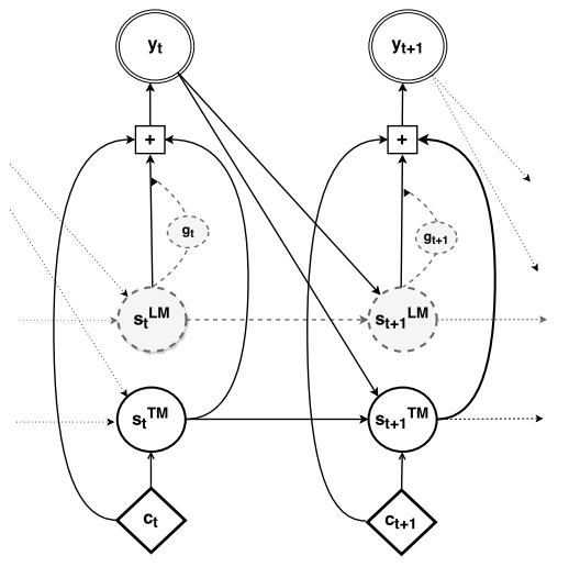
The model is then fine-tuned to use the hidden states from both of these models when computing the output probability of the next word according to the following formula:

\[p\left( y_{t} \middle| y_{< t},\ x \right) \propto \ \exp\left( y_{t}^{T}\left( W_{o}.f_{o}\left( s_{t}^{\text{LM}},\ s_{t}^{\text{NMT}},y_{t - 1},\ c_{t} \right) + b_{o} \right) \right)\]

Where:

$x$ is the input and $y_{< t}$ is all the previous output words.
$y_{t}$ is the suggested output word at time step $t$. Which means that $y_{t - 1}$ is the output word one step before.
$W_{o}$ is the weights of the output layer and $b_{o}$ is the bias.
$f_{o}$ is the activation function of the output layer.
$s_{t}^{\text{LM}}$ is the hidden state of the language model.
$s_{t}^{\text{NMT}}$ is the hidden state of the neural machine translation model.
$c_{t}$ is the context vector produced by the encoder.