MUSE
MUSE or “Multilingual Unsupervised and Supervised Embeddings” is a framework created by Facebook AI in 2017 and published in this paper: Word Translation Without Parallel Data. The official implementation of the framework can be found in this GitHub repository: MUSE.
From the name of the paper, we can see that MUSE is for word translation not machine translation which shows that MUSE is more of a look-up table (bilingual dictionary) rather than being a machine translation model. The crazy part about MUSE is that It builds bilingual dictionary between two languages without the use of any parallel corpora. And despite that it outperforms supervised state-of-the-art methods on English-Italian where metric is the average precision over top 1, 5, 10 words respectively.
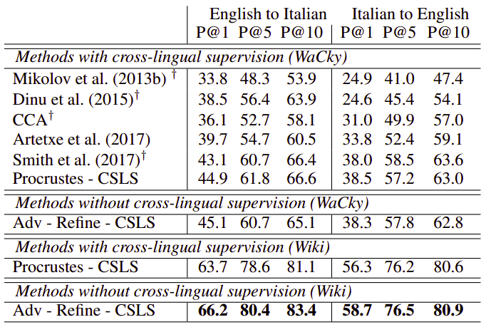
MUSE leverages adversarial training to learn that linear mapping from a source to a target space and it operates in three steps as shown in the following figure where there are two sets of embeddings trained independently on monolingual data, English words in red denoted by $\mathbf{X}$ and Italian words in blue denoted by $\mathbf{Y}$, which we want to align/translate. In this figure, each dot represents a word in that space where the dot size is proportional to the frequency of the words in the training corpus.
MUSE focuses on learning a mapping $\mathbf{\text{WX}}$ between these two sets such that translations are close in the shared space. It does that in three steps:
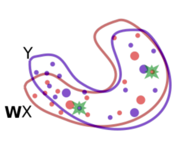
- Adversarial Model:
Using adversarial learning, we learn a rotation matrix $\mathbf{W}$ which roughly aligns the two distributions. The green stars are randomly selected words that are fed to the discriminator to determine whether the two word embeddings come from the same distribution.
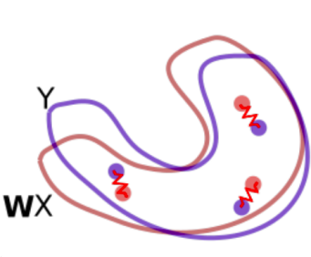
- Refinement Procedure:
The mapping $\mathbf{W}$ is further refined via Procrustes. This method uses frequent words aligned by the previous step as anchor points, and minimizes an energy function that corresponds to a spring system between anchor points. The refined mapping is then used to map all words in the dictionary.
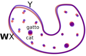
- CSLS:
Finally, we translate by using the mapping $\mathbf{W}$ and a distance metric (CSLS) that expands the space where there is high density of points (like the area around the word “cat”), so that “hubs” (like the word “cat”) become less close to other word vectors than they would otherwise.
Adversarial Model
Let $X = \left\{ x_{1},\ …x_{n} \right\}$ and $Y = \left\{ y_{1},\ …y_{m} \right\}$ be two sets of $n$ and $m$ word embeddings coming from a source and a target language respectively. An adversarial setting formed as a two-player game where the two players are:
- Discriminator:
A classification model trained to distinguish between the mapped source embeddings $\mathbf{W}\mathbf{X}$ and the target embeddings $\mathbf{Y}$. The discriminator aims at maximizing its ability to identify the origin of an embedding.
- W Mapping:
(Which can be seen as a generator) is model jointly trained to fool the discriminator by making $\mathbf{\text{WX}}$ and $\mathbf{Y}$ as similar as possible.
Where:
-
$\mathcal{L}_D$ is the discriminator loss while $\mathcal{L}_W$ is the mapping loss.
-
$\theta_{D}$ is the discriminator parameters.
-
$W$ is the learned linear mapping.
-
$P_{\theta_{D}}\left( \text{source} = 1 \middle| z \right)$ is the probability that a vector $z$ is the mapping of a source embedding. And $P_{\theta_{D}}\left( \text{source} = 0 \middle| z \right)$ is the probability that a vector $z$ is the mapping of a target embedding.
Refinement Procedure
The adversarial approach tries to align all words irrespective of their frequencies. However, rare words are harder to align. Under the assumption that the mapping is linear, it is then better to infer the mapping using only the most frequent words as anchors. The mapping $\mathbf{W}$ is further refined via Procrustes analysis which advantageously offers a closed form solution obtained from the singular value decomposition:
\[W^{*} = \underset{W \in O_{d}\left( \mathbb{R} \right)}{\arg\min}{\left\| WX - Y \right\|_{F} = UV^{T},\ \ \ \ \ \ \text{with }\text{U}\Sigma V^{T} = \text{SVD}\left( YX^{T} \right)}\]This method uses frequent words aligned by the previous step as anchor points, and minimizes an energy function that corresponds to a spring system between anchor points. The refined mapping is then used to map all words in the dictionary.
CSLS
CSLS stands for “Cross-Domain Similarity Local Scaling” which is a novel metric proposed by the authors as a comparison metric between two different language embeddings. Given a mapped source word embedding $Wx_{s}$ and a target embedding $y_{t}$, the CSLS can be formulated as:
\[\text{CSLS}\left( Wx_{s},\ y_{t} \right) = 2\cos\left( Wx_{s},\ y_{t} \right) - r_{T}\left( Wx_{s} \right) - r_{S}\left( y_{t} \right)\] \[r_{T}\left( Wx_{s} \right) = \frac{1}{K}\sum_{y_{t} \in \mathcal{N}_{T}\left( Wx_{s} \right)}^{}{\cos\left( Wx_{s},\ y_{t} \right)}\] \[r_{S}\left( y_{t} \right) = \frac{1}{K}\sum_{Wx_{s} \in \mathcal{N}_{S}\left( y_{t} \right)}^{}{\cos\left( Wx_{s},\ y_{t} \right)}\]Note that all $K$ elements of $\mathcal{N}_{T}\left( Wx_{s} \right)$ are words from the target language and all $K$ elements of $\mathcal{N}_{S}\left( y_{t} \right)$ are mapped words from the source language.
Training Details
-
They used unsupervised word vectors that were trained using fastText.
-
These correspond to monolingual embeddings of dimension 300 trained on Wikipedia corpora; therefore, the mapping $\mathbf{W}$ has size 300×300.
-
Words are lower-cased, and those that appear less than 5 times are discarded for training.
-
As a post-processing step, they only considered the first 200k most frequent words.
-
For discriminator, they used a MLP with two hidden layers of size 2048, and Leaky-ReLU activation functions with dropout of 0.1 trained using stochastic gradient descent with a batch size of 32, a learning rate of 0.1 and a decay of 0.95 both for the discriminator and W mapping.