Analyzing M4 using SVCCA

Multilingual Neural Machine Translation (MNMT) models have yielded large empirical success in transfer learning settings. However, these black-box representations are poorly understood, and their mode of transfer remains elusive. This paper “Investigating Multilingual NMT Representations at Scale” published by Google in 2019 attempted to understand MNMT representations (specifically Google’s M4 model) using Singular Value Canonical Correlation Analysis (SVCCA). Google’s unofficial code for the SVCCA framework can be found on their official GitHub repository: google/svcca.

SVCCA Recap

As mentioned earlier, SVCCA stands for “Singular Value Canonical Correlation Analysis” which is a technique to compare vector representations in a way that is both invariant to affine transformations and fast to compute. This framework was proposed by Google Brain in 2018 and published in this paper: SVCCA: Singular Vector Canonical Correlation Analysis for Deep Learning Dynamics and Interpretability. The following is how SVCCA works.

For a given dataset of $n$ examples $X = \left\{ x_{1},\ …\ x_{n} \right\}$, $z_{i}^{l} \in \mathbb{R}^{n}$ is defined as a vector of the neuron $i$ values of layer $l$ in a neural network across all examples. Note that this is a different vector from the often-considered "layer representation" vector of a single point. Within this formalism, the Singular Vector Canonical Correlation Analysis (SVCCA) proceeds as follows:

SVCCA takes as input two (not necessarily different) sets of neurons (typically layers of a network):

\[l_{1} = \left\{ z_{1}^{l_{1}},\ ...z_{n}^{l_{1}} \right\},\ \ \ \ \ l_{2} = \left\{ z_{1}^{l_{2}},\ ...z_{n}^{l_{2}} \right\}\]

First, SVCCA performs a Singular Value Decomposition (SVD) of each subspace to get smaller dimension while keeping $99\%$ of the variance.

\[{l'}_{1} = SVD\left( l_{1} \right) = \left\{ {z'\ }_{1}^{l_{1}},\ ...{z'\ }_{n_{1}}^{l_{1}} \right\},\ \ where\ n_{1} < n\] \[{l'}_{2} = SVD\left( l_{2} \right) = \left\{ {z'\ }_{1}^{l_{2}},\ ...{z'\ }_{n_{2}}^{l_{2}} \right\},\ \ where\ n_{2} < n\]

Then, SVCCA uses the Canonical Correlation Analysis (CCA) to linearly transform ${l’}_1$ and ${l’}_2$ to be as aligned as possible. CCA is a well established statistical method for understanding the similarity of two different sets of random variables. It does that by linearly transform (${l’}_1$ and ${l’}_2$) vectors to another vectors (${\widetilde{l}}_1$ and ${\widetilde{l}}_2$) where the correlation $corr = \left\{ \rho_1,\ …\rho_{\min\left( n_1, n_2 \right)} \right\}$ is maximized:

\[{\widetilde{l}}_{1} = W_{1}{l'}_{1} = \left\{ {\widetilde{z}}_{1}^{l_{1}},\ ...{\widetilde{z}\ }_{n_{1}}^{l_{1}} \right\}\] \[{\widetilde{l}}_{2} = W_{2}{l'}_{2} = \left\{ {\widetilde{z}}_{1}^{l_{2}},\ ...{\widetilde{z}\ }_{n_{2}}^{l_{2}} \right\}\]

With these steps, SVCCA outputs pairs of aligned directions, (${\widetilde{z}}_i^{l_1}$ , ${\widetilde{z}}_i^{l_2}$) and how well they correlate, $\rho_i$.

Now that we have reviewed what SVCCA is all about; let’s get back to the paper and see how they used SVCCA. In the paper, they applied SVCCA on the sentence-level of the hidden representation of Google’s M4 model averaging over the sequence time-steps.

More concretely, given a batch of size $B$ sentences of max length $T$ in a certain language, the hidden representation of any layer of this MNMT model will be a tensor of $(B \times T \times C)$ dimension where $C$ is the model’s dimension. Applying an average pooling operation on the time-steps (sentence length) will result in a matrix of $(B \times C)$ dimension. This is equivalent to assuming that every token in a sentence from language A is equally likely to be aligned to each token in an equivalent sentence in language B.

MNMT Learns Language Similarity

Using the top-layer of the encoder of Google’s M4 model, they have clustered all languages together based on their SVCCA similarities. Then, they used the “Laplacian Eigenmaps” algorithm implemented in scikit-learn as sklearn.SpectralEmbedding method to visualize these similarities across all languages found in the dataset that was used to train Google’s M4. This dataset is an English-centric dataset containing sentences in 103 languages. The following figure is the result:

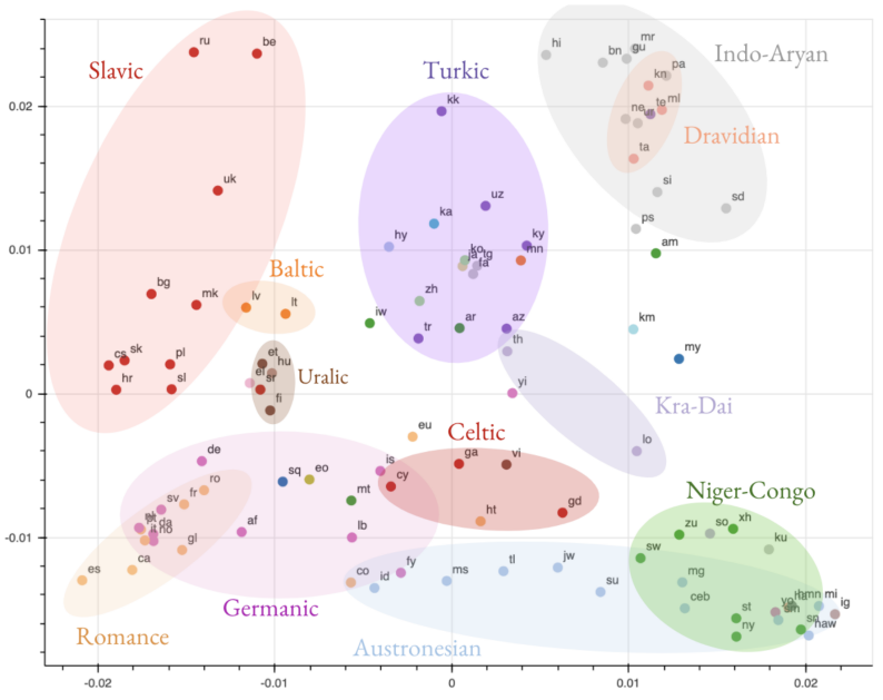
From analyzing these similarities, they have observed remarkable findings:

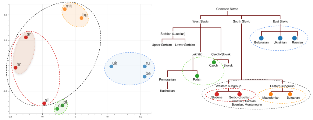
The resulting clusters are grouped not only by the language-family (e.g. Slavic), but also by branches within the language-family (e.g. South Slavic), branches within those branches (e.g. Western Subgroup), and dialects within those (e.g. Serbo-Croatian). The following figure is a visualization of the Slavic languages:

Clustering captures the linguistic similarity between languages (sharing similar grammatical properties) and the lexical similarity (having the same alphabet/scripts and thus sharing many subwords). However, the the lexical similarity gets weaker as we move up on the encoder level. The following figure shows the representations of the Turkic and Slavic languages; within each family there are languages that are written in Cyrillic and Roman alphabets. As you can see languages that use Cyrillic-scripts (blue) are clustered together according to the first encoder layer’s representation. However, they get closer to the Roman-scripts languages (orange) at the last encoder layer’s representation.

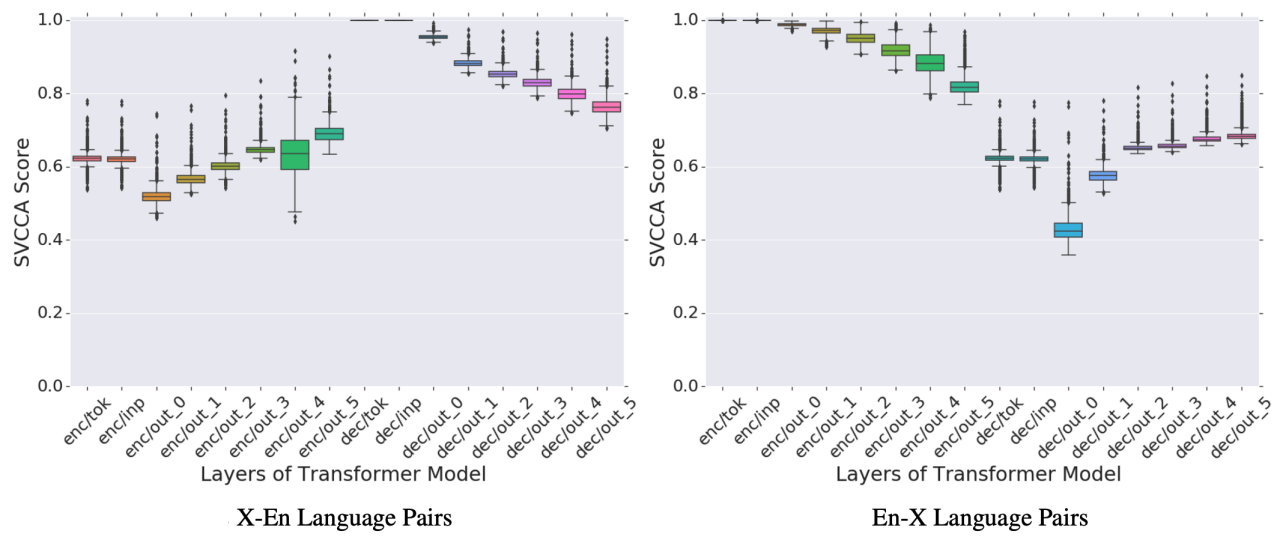
Similarity evolves across encoder/decoder Layers. For each layer, they first computed the pair-wise similarity between all pairs of languages. Then, they aggregated these score into a distribution and represented in the following figures.
- As seen in the X-to-English (left) figure:
  - On the encoder side: the similarity between the source languages (X) increase as we move up the encoder layer, suggesting that the encoder attempts to learn a common representation for all source languages. However, representations at the last layer of the encoder are far from being perfectly aligned.
  - On the decoder side: as the decoder incorporates more information from the source language (X), representations of the target (En) diverge. This is in line with some findings that show that the translated text is predictive of the source language.
- For English-to-Any (right) figure: We observe a similar trend where representations of the source language (En) diverge as we move up the encoder. Same as it happens with the decoder of the left figure.