CTC

Data sets for speech recognition are usually a dataset of audio clips and corresponding transcripts. The main issue in these datasets is that we don’t know how the characters in the transcript align to the audio. Without this alignment, it would be very hard to train a speech recognition model since people’s rates of speech vary. CTC provides a solution to this problem.

CTC stands for “Connectionist Temporal Classification” which is a way to get around not knowing the alignment between the input and the output. CTC was proposed by Alex Graves, Santiago Fernandes, Faustino Gomez, and Jürgen Schmidhuber in 2006 and published in this paper: Connectionist Temporal Classification: Labelling Unsegmented Sequence Data with Recurrent Neural Networks.

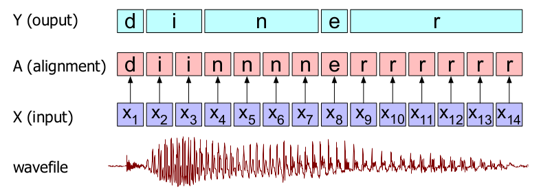
The intuition of CTC is to convert the speech recognition problem to a Temporal Classification problem where each frame of the input audio will be labeled independently to a single character, so that the output will be the same length as the input. Then, a collapsing function that combines sequences of identical letters is applied, resulting in a shorter sequence as shown in the following figure:

Blank Character

The previous figure represents the temporal classification of the audio of someone saying the word “dinner”. Of course, here we are assuming there is a classifier that is able to choose the most probable letter for each input spectral frame representation $x_{i}$ . The sequence of letters corresponding to each input frame is called an “alignment”, because it tells us where in the acoustic signal each letter aligns to. Then, a collapsing function that combines similar letters is applied to result in the word “diner”. As we can see from the past example, this naive algorithm has two problems:

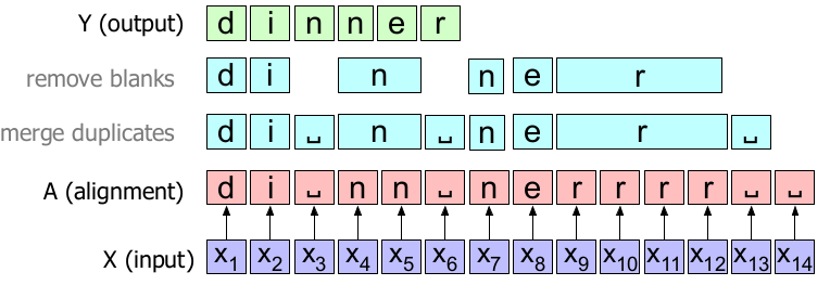
• It doesn’t handle double letters as it transcribed the speech as “diner”, not “dinner”!

• It doesn’t tell us what symbol to align with silence in the input. We don’t want to be transcribing silence as random letters!

The CTC algorithm solves both problems by adding to the transcription alphabet a special symbol for a blank, which we’ll represent as ␣. The blank can be used to separate duplicate characters or to transcribe a silence. Now, the output becomes:

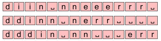
Note: As you probably guessed, the CTC collapsing function has a lot of different alignments that could map to the same output string. The following are just some of the other alignments that would produce the same output and there are many and many more.

Objective Function

To be a bit more formal, let’s consider mapping input sequences$X = \left\lbrack x_{1},x_{2},…,x_{T} \right\rbrack$, such as audio, to corresponding output sequences $Y = \left\lbrack y_{1},y_{2},…,y_{U} \right\rbrack$, such as transcripts. We want to find an accurate mapping from X’s to Y’s. There are challenges which get in the way of us using simpler supervised learning algorithms. In particular:

• Both X and Y can vary in length.

• The ratio of the lengths of X and Y can vary.

• We don’t have an accurate alignment of X and Y.

The CTC algorithm overcomes these challenges. For a given X it gives us an output distribution over all possible Y’s. We can use this distribution either to infer a likely output or to assess the probability of a given output. So, the object function for a single (X, Y) pair is:

where:

• $X$ is a sequence of input data (audio frames for example).

• $Y$ is a sequence of output data (characters for example).

• $p\left( Y \middle| X \right)$: is the CTC conditional probability of output $Y$ given input $X$.

• $\sum_{a \in A_{X,Y}}^{}\ $: is to sum all possible alignments for the $\left( X,Y \right)$ pair alignments.

• $p\left( a_{t} \middle| X \right)$: is the conditional probability of alignment $a$ at time-step $t$ given input sequence $X$.

• $\prod_{t = 1}^{T}\ $: is the probability for a single alignment $a_{t}$ step-by-step over all $T$ steps.

As we can see, we can summarize the objective function as the sum of all possible true alignments for the given input. To understand what that means and how the objective function is calculated, let’s take a simple example where the input $X = \left\lbrack x_{1},x_{2},x_{4},x_{4},x_{5},x_{6} \right\rbrack$ and the true transcribed is “ab”. We can calculate the objective function using the following steps:

• As explained earlier, CTC uses the blank character ␣. So, we need to expand the true output to include that character. Now, the true output becomes:

• Then, we are going to form the CTC network where the number of rows should be the extended output and the number of columns should be the length of the input like so:

• Define all the possible alignments of the previous CTC network:

• Now, the objective function will be the sum of the likelihood of each path of these. In other words, $p\left( Y \middle| X \right)$ will be:

where:

...

Then, the loss function will be just the negative log-likelihood of the objective function. So, for a training $D$, the loss function will be:

CTC Inference

After we’ve trained the model, we’d like to use it to find a likely output for a given input. More precisely, we need to solve:

We can obtain that by considering the most likely output at each time-step greedily. This is called “Greedy Search” and it works well for many applications. However, this approach can sometimes miss easy to find outputs with much higher probability.

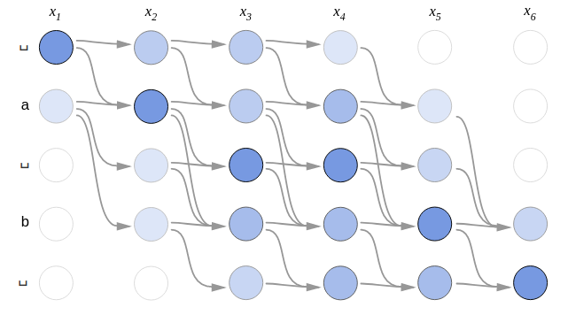
A better approach is to use “Beam Search”. A standard/vanilla beam search computes a new set of hypotheses at each input time-step. The new set of hypotheses is generated from the previous set by extending each hypothesis with all possible output characters and keeping only the top few candidates which is known as “beam size”. The following example uses a beam size of 3.

We can modify the vanilla beam search by the following modifications:

• Instead of keeping a list of alignments in the beam, we merge any alignments that map to the same output.

• Also, remove the blank characters "␣" when encountered.

Now, the paths will be:

Notes:

• The blank character “␣” is like a garbage token, it doesn’t represent anything but noise. So, it’s very different than the space character “ “.

• CTC works only when the output sequence Y is shorter than the input sequence X.

• CTC assumes conditional independence which means that the output at time $t$ is independent of the output at time $t - 1$, given the input.

• CTC does not implicitly learn a language model over the data (except for the case of attention-based encoder-decoder architectures). It is therefore essential when using CTC to interpolate a language model using a hyper-parameter$\lambda$ that is fine-tuned on a dev set:

\[p\left( Y \middle| X \right) = \lambda\log\ p_{\text{CTC}}\left( Y \middle| X \right) + \left( 1 - \lambda \right)\log\ p_{\text{LM}}\left( Y \right)\]

• For more details about implementing CTC, you should check this gist created by Awni Hannun the one who optimized CTC in this paper. And also this one which is talking about prefix Beam Search.