RNN-T: RNN Transducer

RNN-T stands for “Recurrent Neural Network Transducer” which is a promising architecture for general-purpose sequence such as audio transcription built using RNNs. RNN-T was proposed by Alex Graves at the University of Toronto back in 2012 and published under the name: Sequence Transduction with Recurrent Neural Networks. This paper introduces an end-to-end, probabilistic sequence transduction system, based entirely on RNNs, that is in principle able to transform any input sequence into any finite, discrete output sequence.

Let $x = \left( x_{1},\ x_{2},\ …x_{m} \right)$ be a length $m$ input sequence of arbitrary length belonging to the set $X$, and let $y = \left( y_{1},\ y_{2},\ …y_{n} \right)$ be a length $n$ input sequence of arbitrary length belonging to the set $Y$. RNN-T model tries to define the following conditional distribution; where $a$ refers to the alignments between the input and output sequences:

Both the inputs vectors $x_{i}$ and the output vectors $y_{j}$ are represented by fixed-length real-valued vectors where $x_{i}$ would typically be a vector of MFC coefficients and $y_{j}$ would be a one-hot vector encoding a particular phoneme or null $\varnothing$.

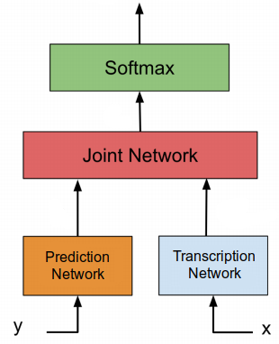
As shown in the past figure, RNN-T consists of three networks to determine the past conditional distribution:

• Transcription Network $F$:
  This RNN network acts like an acoustic model as it scans the input sequence $x$ and outputs the transcription (feature) vector sequence:

• Prediction Network $G$:
  This RNN network acts like a language model as it scans the output sequence $y$ and outputs the prediction vector sequence:

• Joint Network:
  This network is a simple feed-forward network that combines the transcription vector $f_i$ and the prediction vector $g_j$.

Transcription Network

The transcription network $F$ is a bidirectional RNN that scans the input sequence $x$ forwards and backwards with two separate hidden layers, both of which feed forward to a single output layer. Bidirectional RNNs are preferred because each output vector depends on the whole input sequence (rather than on the previous inputs only, as is the case with normal RNNs).

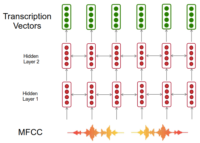
Given a length $m$ input sequence $\left( x_{1}, x_{2}, …x_{m} \right)$, the transcription network $F$ computes the forward hidden sequence $\left( {\overrightarrow{h}}_1, {\overrightarrow{h}}_2, …{\overrightarrow{h}}_m \right)$, the backward hidden sequence $\left( {\overleftarrow{h}}_1, {\overleftarrow{h}}_2, …{\overleftarrow{h}}_m \right)$, and the transcription sequence $\left( f_1, f_2, …f_m \right)$ by first iterating over the backward and forward layer:

Where $W_{i}$, $W_{h}$, and $b_{h}$ are learnable weights for input and hidden layer and hidden bias respectively. Then, it combines the backward and forward vectors to generate output layers:

Note:
In this paper, the $H$ function refers to the type of RNN cell used which is “LSTM”.

Prediction Network

The prediction network $G$ is a recurrent neural network consisting of an input layer, a single hidden layer, and an output layer. The inputs to this network are phonemes encoded as one-hot vectors while the output are the prediction vectors.

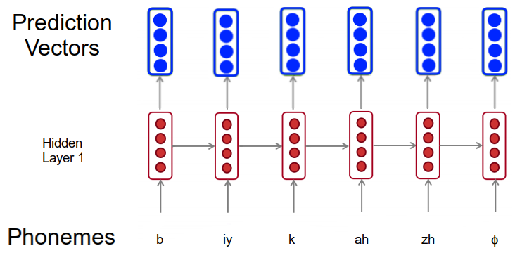
Given a length $n$ phoneme sequence $\left( y_{1},\ y_{2},\ …y_{n} \right)$, the prediction network $G$ computes the hidden sequence $\left( h_{1},\ h_{2},\ …h_{n} \right)$ and the prediction sequence $\left( g_{1},\ g_{2},\ …g_{n} \right)$ by using the following equations:

Where $W_{ih}$ is the input-hidden weight matrix, $W_{hh}$ is the hidden-hidden weight matrix, $W_{ho}$ is the hidden-output weight matrix, $b_{h}$ and $b_{o}$ are the bias terms, and $H$ is the LSTM cell functions.

Joint Network

As said ealier, the Joint network (Joiner) is a simple feed-forward network that combines the transcription vector $f_i$ and the prediction vector $g_j$ and results in the output vector whose size is $K + 1$ where $K$ is the unique characters in the data/language plus the null character ($\varnothing$).

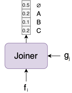
The output from the Joint Network will be the output vector. We can apply $Softmax()$ over that vector to get the most probable character for that time-step or we can use these soft labels and decode it in a smarter way as we are going to see next.

Output Distribution

Now, given the transcription vector $f_{i}$, where $1 \leq i \leq m$, the prediction vector $g_{t}$, where $0 \leq j \leq n$, and a set of labels $K$, we define the output density function as:

Where superscript $k$ denotes the $k^{\text{th}}$ element of the vectors. The density can be normalised to yield the following conditional output distribution:

The probability $pr\left( k \middle| i,\ j \right)$ describes the transition probabilities in the lattice shown in the following figure. In the following figure, the horizontal arrow leaving node $\left( i,j \right)$ represents the probability outputting nothing $\varnothing\left( i,j \right)$; the vertical arrow represents the probability of outputting the element $j + 1$ of $y$. The black nodes at the bottom represent the null state before any outputs have been emitted.

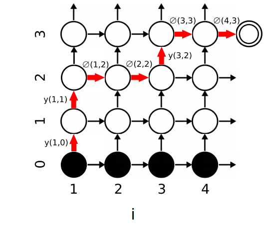
The set of all possible paths from the bottom left to the terminal node in the top right corresponds to the complete set of alignments between audio $x$ and transcription $y$. Each alignment probability is the product of the transition probabilities of the arrows they pass through. To obtain the best alignment (shown in red), the Forward-Backward algorithm is used.

The Forward-Backward Algorithm defines two probabilities

• The forward probability $\mathbf{\alpha}\left( \mathbf{i,j} \right)$: As the probability of outputting $y_{\left\lbrack 1:j \right\rbrack}$ during $f_{\left\lbrack 1:i \right\rbrack}$ where the forward variables can be calculated recursively using the following formula with the initial condition that $\alpha\left( 1,0 \right) = 1$:

• The backward probability $\mathbf{\beta}\left( \mathbf{i,j} \right)$: As the probability of outputting $y_{\left\lbrack j + 1:n \right\rbrack}$ during $f_{\left\lbrack i:m \right\rbrack}$ where the backward variables can be calculated recursively using the following formula with the initial condition that $\beta\left( 1,0 \right) = \varnothing\left( m,n \right)$:

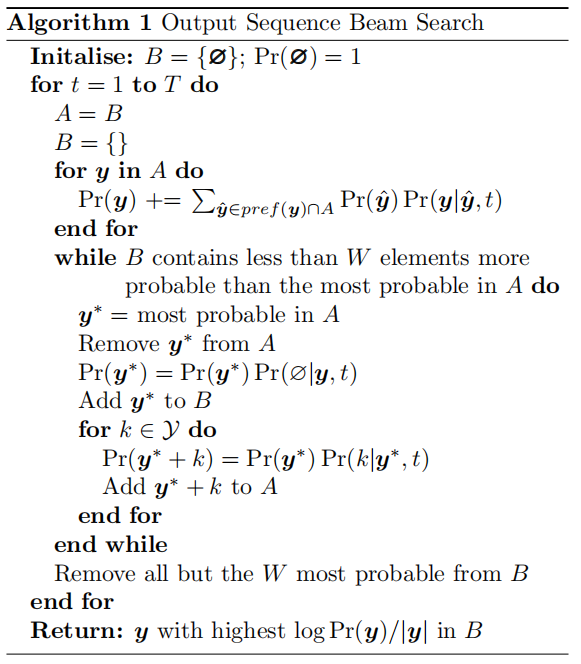
From the definition of the forward and backward probabilities, we can find the best alignment by following their product $\alpha\left( i,j \right)\beta\left( i,j \right)$ at any point $\left( i,j \right)$ in the output lattice using a beam search (defined in the following algorithm):

Experiments

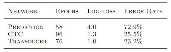
To evaluate the potential of the RNN transducer, they applied it to the task of phoneme recognition on the TIMIT speech corpus. The core training and test sets of TIMIT contain respectively $3696$ and $192$ phonetically transcribed utterances. They defined a validation set by randomly selecting $184$ sequences from the training set. Regarding phonemes, they used the reduced set of $39$ phoneme targets.

Regarding the audio features, they created input sequences of length $26$ normalized to have mean zero and standard deviation one using standard speech preprocessing. For preprocessing, Hamming windows of $25ms$ length at $10ms$ intervals were used.

Regarding the prediction network, they used one hidden layer of LSTM cells of size $128$. Regarding the transcription network, they use two hidden layers of LSTM cells of size $128$. This gave a total of $261,328$ weights in the RNN transducer. As we can see in the following table, the phoneme error rate of the transducer is among the lowest recorded on TIMIT: