Deep Speech 2.0

Deep Speech 2 is a model created by Baidu in December 2015 (exactly one year after Deep Speech) and published in their paper: Deep Speech 2: End-to-End Speech Recognition in English and Mandarin. This paper is considered a follow-on the Deep Speech paper, the authors extended the original architecture to make it bigger while achieving 7× speedup and 43.4% relative improvement in WER. Also, the authors incorporating the convolution layers as shown in the following figure:

The input of this model is a spectrogram frame of size $t$ along with context of C frames on each side. C could be 5, 7, 9 frames on each side. And the activation functions used for this network is a clipped ReLU at 20.

\[g(z) = min\left( \max\left( 0,\ z \right),\ 20 \right)\]

The optimal architecture of Deep Speech 2 is composed of 11hidden layers:

The first three layers are convolutional layers + Batch Normalization where $h_{t,\ i}^{l}$ is the hidden representation at layer $l$ and time-frame $t$ of the $i^{th}$ filter. $w_{i}^{l}$ is the weights of the $i^{th}$ fitler at layer $l$. $\circ$ denotes an element-wise product and $c$ is the context window size:

\[h_{t,\ i}^{l} = g\left( w_{i}^{l} \circ h_{t - c:t + c}^{l - 1} \right)\]

The next seven layers are bidirectional RNN layers + Batch Normalization where is $\overrightarrow{h_{t}^{l}}$ the forward path and $\overleftarrow{h_{t}^{l}}$ is the backward path at time-frame $t$ at layer $l$. Wl is the input-hidden weight matrix, $\overrightarrow{U^{l}}$ is the forward recurrent weight matrix, $\overleftarrow{U^{l}}$ is the backward recurrent weight matrix, and $b^{l}$ is a bias term:

\[\overrightarrow{h_{t}^{l}} = g\left( W^{l}h_{t}^{l - 1} + \overrightarrow{U^{l}}\ {\overrightarrow{h}}_{t - 1}^{l} + b^{l} \right)\] \[\overleftarrow{h_{t}^{l}} = g\left( W^{l}h_{t}^{l - 1} + \overleftarrow{U^{l}}\ {\overleftarrow{h}}_{t - 1}^{l} + b^{l}\ \right)\] \[h_{t}^{l} = \overrightarrow{h_{t}^{l}} + \overleftarrow{h_{t}^{l}}\]

The last layer is just a fully connected layer).

\[h_{t}^{l} = g\left( W^{l}h_{t}^{l - 1} + b^{l} \right)\]

The output layer is a standard Softmax function that yields the predicted character probabilities for each time slice (t) and character k in the alphabet:

\[h_{t,k}^{(11)} = p\left( c_{t} = k \middle| x \right) = \frac{\exp\left( W_{k}^{(11)}h_{t}^{(10)} \right)}{\sum_{j}^{}{\exp\left( W_{j}^{(11)}h_{t}^{(10)} \right)}}\]

Researchers of Deep Speech 2 explored many different architectures; varying the number of recurrent layers from 1 to 7 with both RNN and GRU architecture while using just one 1D convolutional layer; and the following table shows the effect on WER:

They also tried varying the number of convolutional layers between 1 and 3 with both RNN and GRU while using 7 layers of RNN cells; and the following table shows the effect on WER:

And the optimal architecture for English transcription was the one introduced earlier.

Model Details

The following are the details that were used to train the deep speech 2 model:

The model uses a vocabulary of (a, b, c, ..., z, space, apostrophe, blank) for English. They have added the apostrophe as well as a space symbol to denote word boundaries.
The model uses CTC loss.
The model uses synchronous SGD as an optimizer.
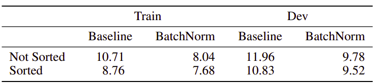
The model uses SortaGrad which is a technique to batch utterances based on the length, so longer utterances will be in the same batch. Then, in the first epoch, we iterate over the training data in increasing order of the length of utterances in the minibatch. After the first epoch, training reverts back to a random order over minibatches. The following table shows the effect of that technique over the WER:

The model was trained using around 11,940 hours. They, even, augmented the training data by adding noise to 40% of the utterances randomly.

The following are the details that were used for inference:
The model uses a beam search algorithm with a typical beam size in the range 500 for English and 200 for Mandarin.
The model uses 5-gram language model smoothed using Kneser-Ney method and it was trained on 400,000 words from 250 million lines of text collected from the Common Crawl Repository.
The following formula is used to get the best sequence of words where $x$ is the context, $c$ is the characters sequence, $\alpha$ and $\beta$ are tunable parameters that controls the trade-off between the acoustic model, the language model.

\[Q(c) = log\left( \mathbb{P}\left( c \middle| x \right) \right) + \alpha\ \log\left( \mathbb{P}_{\text{lm}}(c) \right) + \beta\ word\_ count(c)\]