Tacotron
Tacotron is a two-staged generative text-to-speech (TTS) model that synthesizes speech directly from characters. Given (text, audio) pairs, Tacotron can be trained completely from scratch with random initialization to output spectrogram without any phoneme-level alignment. After that, a Vocoder model is used to convert the audio spectrogram to waveforms. Tacotron was proposed by Google in 2017 and published in this paper under the same name: Tacotron: Towards End-to-End Speech Synthesis. The official audio samples outputted from the trained Tacotron by Google is provided in this website. The unofficial TensorFlow implementation for Tacotron can be found in this GitHub repository: tacotron.
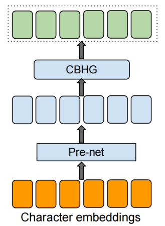
As we can see from the Tacotron architecture illustrated below, Tacotron consists of four main components: an Encoder, a Decoder, an Attention Mechanism, and a Post-processing Network.

Encoder
The goal of the encoder is to extract robust sequential representations of text. As you can see from the encoder’s architecture:
-
The input to the encoder is a character sequence, where each character is represented as a one-hot vector and embedded into a continuous vector.
-
Each of these character emeddings is passed to the “pre-net” block which is basically a non-linear bottleneck layer with dropout. This network helps with convergence and improves generalization.
-
Finally, the output from the pre-net is passed to the CBHG network (we are going to talk about it in more details later). The CBHG network transforms the pre-net outputs into the final encoder representation used by the attention module. In the paper, they found that using this module not only reduces overfitting, but also makes fewer mispronunciations.
Decoder + Attention Mechanism
The goal of the decoder and the attention mechanism is to align the audio frames with the textual features outputted from the encoder and result in audio spectrogram. As shown in the following figure, the decoder works like the following:
-
The first decoder step is conditioned on an all-zeros frame (the <GO> frame).
-
The input frame is passed to a pre-net block as done in the encoder. The pre-net block, as stated earlier, is a non-linear bottleneck layer combined with a dropout mechanism.
-
The output of the pre-net block is passed to a tanh attention RNN layer. The output from this layer is concatenated with the context vector from the attention mechanism to form the input to the decoder RNNs.
-
The output from the decoder RNNs is passed to a simple fully-connected output layer to predict the decoder targets, each decoder target is a combination of $r$ 80-band mel-scale spectrogram frames at once. Doing so reduces the model size, training time, and inference time. Also, they found that this also helps with convergence.
-
During inference, at decoder step $t$, the last frame of the $r$ predictions is fed as input to the decoder at step $t + 1$. Note that feeding the last prediction is just a decision they made in the paper, they could have used all $r$ predictions.
Note:
They used 256 GRU cells in all RNN layers, they tried LSTM and obtained similar results. Also, residual connections were used between layers, which sped up convergence.

Post-processing Network
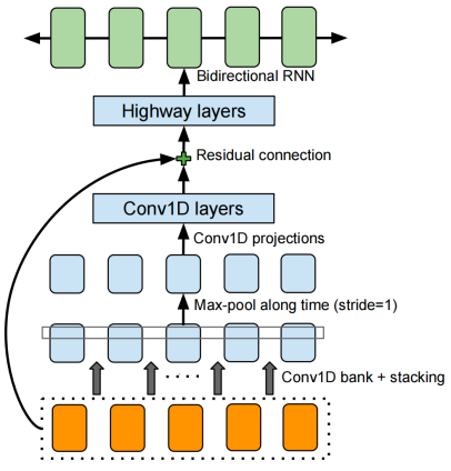
The goal of the post-processing net is to convert the decoder’s target into waveforms. The need for a whole network to do this task is the need to see the full decoded sequence instead of doing it auto-regressively. The backbone of this network is the CBHG (Convolution Bank + Highway GRU) network which consists of a bank of 1-D convolutional filters, followed by highway networks and a bidirectional GRU layer. It works like so:
-
The input sequence is first convolved with $K$ sets of 1-D convolutional filters, where the $k^{\text{th}}$ set contains $C_{k}$ filters of width $k$. These filters explicitly model local and contextual information (akin to modeling unigrams, bigrams, up to K-grams).
-
The convolution outputs are stacked together and further max pooled along time-axis to increase local invariances. Note that they used a stride of $1$ to preserve the original time resolution.
-
Then, the processed sequence is passed to a few fixed-width 1-D convolutions, whose outputs are added with the original input sequence via residual connections. Batch normalization was used for all convolutional layers.
-
The convolution outputs are fed into a multi-layer highway network to extract high-level features.
-
Finally, a bidirectional GRU RNN is added on top to extract sequential features from both forward and backward context.
After the CBHG network, two more steps were applied as shown in the following figure of the post-processing network:

-
The output from the CBHG network is raised by a power of $1.2$. Doing so reduces artifacts, likely due to its harmonic enhancement effect.
-
Then, these scaled spectrogram frames are fed to the Griffin-Lim algorithm to synthesize waveform. They didn’t use any loss function for this part of the model since this algorithm doesn’t have any trainable weights.
Note:
In the paper, the authors said that their choice of Griffin-Lim algorithm is just for simplicity; while it already yields strong results, developing a fast and high-quality trainable spectrogram to waveform inverter is ongoing work.
Experiments
In the paper, they trained Tacotron on an internal North American English dataset, which contains about 24.6 hours of speech data spoken by a professional female speaker. The phrases are text normalized, e.g. “16” is converted to “sixteen”. The audio data were sampled to $24kHz$. Also, they used log magnitude spectrogram with Hann windowing, $50\ ms$ frame length, $12.5\ ms$ frame shift, and 2048-point Fourier transform and 0.97 pre-emphasis.
For training Tacotron, they used $r = 2$ (output layer reduction factor), though larger $r$ values (e.g. $r = 5$) also work well. They used a batch size of 32. Training was done usingAdam optimizer with learning rate decay, which starts from $0.001$ and is reduced to $0.0005$, $0.0003$, and $0.0001$ after $500K$, $1M$ and $2M$ global steps, respectively. They used a simple L1 loss for both seq2seq decoder (mel-scale spectrogram) and post-processing net (linear-scale spectrogram). The two losses have equal weights. The full list of the hypter-parameters used can be found in the following table:

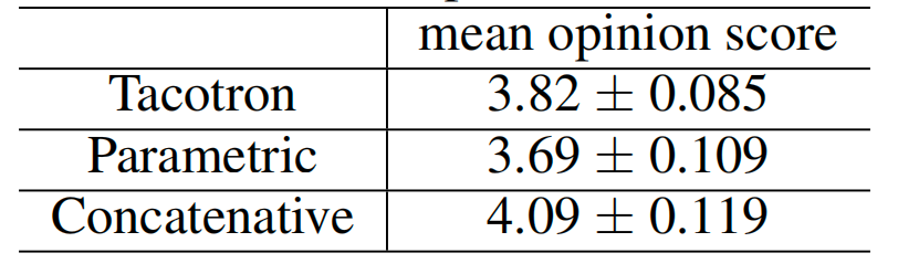
To evaluate the model, they conducted mean opinion score (MOS) tests, where the subjects were asked to rate the naturalness of the stimuli in a 5-point Likert scale score. The MOS tests were crowd-sourced from native speakers. 100 unseen phrases were used for the tests, and each phrase received 8 ratings.
In the paper, they compared Tacotron with a parametric (based on LSTM) model from this paper: Fast, Compact, and High Quality LSTM-RNN Based Statistical Parametric Speech Synthesizers for Mobile Devices; and a concatenative system from this paper: Recent advances in Google real-time HMM-driven unit selection synthesizer. As shown in the following table, Tacotron achieves an MOS of 3.82 which is a very promising result: