Word2Vec
Word2Vec stands for “word-to-vector” is a model architecture created by Tomáš Mikolov from Google in 2013 and published in the paper: Efficient Estimation of Word Representations in Vector Space. This model aims at computing continuous vector representations of words from very large data sets.
It uses a principle in distributional semantics that says that “the word’s meaning is given by the words that frequently appear close-by”. And this is the main idea behind “word2vec”. Also, this means that similar words will appear in similar context which will make their vectors similar and that’s a great feature in word2vec as we are going to see later.
The way we define these vectors is actually a trick you may have seen elsewhere in machine learning. We’re going to train a simple neural network with a single hidden layer to perform a certain task, but then we’re not actually going to use that neural network for the task we trained it on! Instead, the goal is actually just to learn the weights of the hidden layer, these weights are actually the “word vectors” that we’re trying to learn.
So now we need to talk about this “fake” task that we’re going to build the neural network to perform, and then we’ll come back later to how this indirectly gives us those word vectors that we are really after. We’re going to train the neural network to be a language model. To be more specific, the model should do the following; given nearby words (before and after), the model should predict the most probable word that fits. At first, it will be random but after a few iterations over the training data it will produce more appropriate results. When we say "nearby", there is actually a "window size" parameter to the algorithm. A typical window size might be 5, meaning 5 words behind and 5 words ahead (10 in total).
Word2vec comes in two flavors, the Continuous Bag-of-Words model (CBOW) and the Skip-Gram model. Algorithmically, these models are similar, except for only one thing which is the shape of the input layer and the output layer. As CBOW predicts target words from source context words, while the skip-gram does the inverse and predicts source context-words from the target words.
This inversion might seem like an arbitrary choice, but statistically it has the effect that CBOW smooths over a lot of the distributional information (by treating an entire context as one observation). For the most part, this turns out to be a useful thing for smaller datasets. However, skip-gram treats each context-target pair as a new observation, and this tends to do better when we have larger datasets.
I know this seems difficult, so let’s see the Skip-Gram and CBOW models in more details.
Skip-Gram
Skip-Gram model is a model and how to prepare the training data. In Skip-Gram, we’ll train the neural network by feeding it word pairs found in our training documents. The below example shows some of the training samples (word pairs) we would take from the sentence “The quick brown fox jumps over the lazy dog”. Here, we’ve used a small window size of $2$ just for the example. A more reasonable size would be $5$ or more. The word highlighted in blue is the input word (center) and the other two on the left and right are the context words, each is called (target).
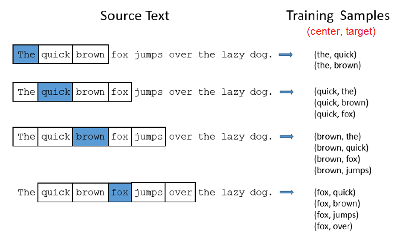
The network is going to learn the statistics from the number of times each pairing shows up. So, for example, the network is probably going to get many more training samples of (“Soviet”, “Union”) than it is of (“Soviet”, “Apple”). When the training is finished, if you give it the word “Soviet” as input, then it will output a much higher probability for “Union” or “Russia” than it will for “Apple”.
Now, how is this all represented? First of all, we know we can’t feed a word just as a text string to a neural network, so we need a way to represent the words to the network. To do this, we first build a vocabulary of words from our training documents, let’s say we have a vocabulary of $10,000$ unique words. Then, we’re going to represent the input word as a one-hot vector. This vector will have $10,000$ components (one for every word in our vocabulary) and we’ll place a $1$ in the position corresponding to the word, and $0$s in all of the other positions.
The output of the network is a single vector (also with $10,000$ components) containing, for every word in our vocabulary, the probability that a randomly selected nearby word is that vocabulary word. Here’s the architecture of our neural network, noting that there is no activation function on the hidden layer neurons, but the output neurons use Softmax:

When training this network on word pairs, the input is a one-hot vector representing the input word and the training output is also a one-hot vector representing the output word. But when we evaluate the trained network on an input word, the output vector will actually be a probability distribution (i.e., a bunch of floating point values, not a one-hot vector).
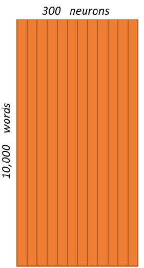
For our example, we’re going to say that we’re learning word vectors of $300$ features. So the hidden layer is going to be represented by a weight matrix of $10,000$ rows (one for every word in our vocabulary) and $300$ columns (one for every hidden neuron). “$300$ features” is what Google used in their published model trained on the Google news dataset, but we can tune this number if we want; we can try different values and see what yields the best results. As a matter of fact, the weights of the hidden layer after finishing training, is the word embedding we are looking for. This matrix is often called “Embedding Matrix”
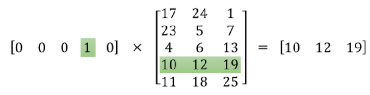
So, the end goal of all of this is really just to learn this hidden layer weight matrix, the output layer we’ll just toss when we’re done! Let’s get back, though, to working through the definition of this model that we’re going to train. The one-hot vector is almost all zeros, what’s the effect of that? If we multiply a $1 \times 10,000$ one-hot vector by a $10,000 \times 300$ matrix, it will effectively just select the matrix row corresponding to the 1. This means that the hidden layer of this model is really just operating as a lookup table.
Here’s a small example to give you a visual:
The output layer is a Softmax regression classifier of $10,000$ neurons. Each output neuron has a weight vector which it multiplies against the word vector from the hidden layer, then it applies the Softmax activation function. Here’s the formula that we are going to follow to train this neural network:
\[p\left( \text{target} \middle| \text{context} \right) = \frac{\exp\left( u_{\text{target}}^{T}.v_{\text{context}} \right)}{\sum_{i = 1}^{V}{\exp\left( u_{i}^{T}.v_{\text{context}} \right)}}\]Such that:
-
$\text{target}$ is the target word.
-
$\text{target}$ is the context word.
-
$V$ is the number of words in our vocabulary.
-
$u_{\text{target}}$ refers to the word vector of the target word. Its shape should be $d \times 1$ where $d$ is the number of features/dimensions ($300$ in our case). $u_{\text{target}}^{T}$ shape should be $1 \times d$.
-
$v_{\text{context}}$ refers to the output-layer vector (outside vector) of the context word. Its shape should be $1 \times d$ where $d$ is the number of features ($300$ in our case).
So, as we can see each word has two representations in our Word2Vec model; one when it’s a target word and another when it’s a context word. Here’s an illustration of calculating the output of the output neuron for an input word.

If two different words have very similar contexts, then our model needs to output very similar results for these two words. So, if two words have similar contexts, then our network is motivated to learn similar word vectors for these two words. And what does it mean for two words to have similar contexts? I think we could expect that synonyms like “intelligent” and “smart” would have very similar contexts. Or that words that are related, like “engine” and “transmission”, would probably have similar contexts as well. This can also handle stemming for us – the network will likely learn similar word vectors for the words “ant” and “ants” because these should have similar contexts. The following formula is cost function that we are going to use to learn our model:
\[J = \frac{- 1}{S}\sum_{i = 1}^{S}\left( \sum_{- m \leq j \leq m,j \neq 0}^{}{\log\left( p\left( w_{i + j} \middle| w_{i} \right) \right)} \right)\]Such as that:
-
$J$ represents the objective function.
-
$S$ represents the total number of sentences that we are going to train our model upon.
-
$m$ is the window size.
-
$w_{i}$ is the context word.
-
$w_{j + i}$ is the target word.
-
$p\left( w_{i + j} \middle| w_{i} \right)$ represents the probability of the target word given the context word. In other words, it’s equal to:
You may have noticed that the skip-gram neural network contains a huge number of weights. For our example with $300$ features and a vocab of $10,000$ words, that’s $3,000,000$ weights in the hidden layer and output layer each! Running gradient descent on a neural network that large is going to be slow. And to make matters better, you need a huge amount of training data in order to tune that many weights and avoid over-fitting. Millions of weights times billions of training samples means that training this model is going to be a beast. The authors of Word2Vec addressed these issues in their second paper: “Distributed Representations of Words and Phrases and their Compositionality”.
There are three innovations in this second paper that made training a bit faster:
-
Treating common word pairs or phrases as single “words” in their model.
-
Subsampling frequent words to decrease the number of training examples.
-
Modifying the optimization objective with a technique they called “Negative Sampling”, which causes each training sample to update only a small percentage of the model’s weights. It’s worth noting that subsampling frequent words and applying Negative Sampling not only reduced the compute burden of the training process, but also improved the quality of their resulting word vectors as well.
Let’s talk about these three modifications with more details:
Word Pairs
Here, we are going to explain the first innovation (or modification) that the authors of Word2Vec have produced in their second paper. The authors pointed out that a word pair like “Boston Globe” (a newspaper) or “Chicago Bulls” (a Basketball Team) has a much different meaning than the individual words “Chicago” and “Bulls”. So it makes sense to treat them as a single word with its own word vector representation. We can see the results in their published model, which was trained on $100$ billion words from a Google News dataset. The addition of phrases to the model swelled the vocabulary size to $3$ million words!
But the question here is “how did they detect these word-pairs?”. The answer is very straight forward. Each pass of their model only looks at combinations of two words, but you can run it multiple times to get longer phrases. So, the first pass will pick up the phrase “New_York”, and then running it again will pick up “New_York_City” as a combination of “New_York” and “City” and so on. The tool counts the number of times each combination of two words appears in the training text, and then these counts are used in an equation to determine which word combinations to turn into word-pair.
The equation is designed to pay attention to the word-pairs that occur together often relative to the number of individual occurrences. It also favors pairs made of infrequent words in order to avoid making phrases out of common words like “and the” or “this is”.
Subsampling Frequent Words
We have seen how training samples were created from the source text. The below example shows some of the training samples (word pairs) we would take from the sentence “The quick brown fox jumps over the lazy dog.” using a small window size of 2. The word highlighted in blue is the input word:

But, in this representation we have two problems with common words like “the”:
-
When looking at word pairs, (“fox”, “the”) doesn’t tell us much about the meaning of “fox”. “the” appears in the context of pretty much every word.
-
We will have many more samples of (“the”, …) than we need to learn a good vector for “the”.
Word2Vec implements a “subsampling” scheme to address this. They implemented an equation for calculating a probability with which to keep a given word in the vocabulary. This probability that we cut the word is related to the word’s frequency as we can see:
\[P\left( w_{i} \right) = \frac{\left( \sqrt{\frac{z\left( w_{i} \right)}{s}} + 1 \right) \ast s}{z\left( w_{i} \right)}\]Where $w_{i}$ represent the word, $z\left( w_{i} \right)$ represents the word frequency ratio. For example, if the word “peanut” occurs $1,000$ times in a one-billion-word corpus, then $z\left( ‘peanut’ \right) = \frac{10^{3}}{10^{9}} = 10^{- 6}$. And $s$ is the ‘sampling rate’ which is a hyper-parameter that controls how much subsampling occurs, and the default value is $0.001$. Smaller values of ‘sampling rate’ mean words are less likely to be kept. And finally, $P\left( w_{i} \right)$ represents the probability of keeping the word $w_{i}$.
Now, if we have a window size of 10, and we remove a specific instance of “the” from our text. Then, we will train on the remaining words, as “the” will not appear in any of their context windows. And we’ll have 10 fewer training samples where “the” is the input word.
Negative Sampling
Training a neural network means taking a training example and adjusting all of the neuron weights slightly so that it predicts that training sample more accurately. In other words, each training sample will tweak all of the weights in the neural network. As we discussed above, the size of our word vocabulary means that our Skip-Gram neural network has a tremendous number of weights, all of which would be updated slightly by every one of our billions of training samples!
Negative sampling addresses this by having each training sample only modify a small percentage of the weights, rather than all of them. Here’s how it works:
- When training the network on the word pair (“fox”, “quick”), we will generate another $k$ words randomly from the vocabulary. These $k$ words are called negative samples. The paper says that selecting 5-20 words works well for smaller datasets, and you can get away with only 2-5 words for large datasets.

As we can see, here we have generated $4$ words randomly from the vocabulary and they are (“king”, “orange”, “box”, and “the”). As we can see, the word “the” exists in the context of the word “quick”, but it’s ok.
- After that, we will multiply the Embedding Matrix $E$ by the one-hot vector of the five words producing embedding vector:
- Finally, change the problem into a classification problem where the input is the word-pairs; and the output is either 1 or zero.
Recall that the output layer of our model has a weight matrix of $300 \times 10,000$. So, we will just be updating the weights for our positive word (“quick”), plus the weights for $4$ other words that we want to output 0. That’s a total of $5$ output neurons, and $1,500$ weight values total. That’s only $0.06\text{\%}$ of the $3$ Million weights in the output layer!
Choosing the “negative samples” randomly isn’t that efficient because the probability of a common word like “and” to be chosen is higher than any other word. Instead, we use a “unigram distribution” where the probability for selecting a word as a negative sample is related to its frequency, with more frequent words being more likely to be selected as negative samples as we can see in the following formula:
\[P\left( w_{i} \right) = \frac{f\left( w_{i} \right)^{\frac{3}{4}}}{\sum_{j = 0}^{n}\left( f\left( w_{i} \right)^{\frac{3}{4}} \right)}\]Where $P\left( w_{i} \right)$ represents the probability of a word $w_{i}$ to be selected as a negative sample. As we can see, each word is given a weight equal to its frequency (word count) $f\left( w_{i} \right)$ raised to the $\frac{3}{4}$ power. The decision to raise the frequency to the $\frac{3}{4}$ power appears to be experiential
\[J = \frac{1}{S}\sum_{i = 1}^{S}\left( \sum_{- m \leq j \leq m,j \neq 0}^{}{\log\left( p\left( w_{i + j} \middle| w_{i} \right) \right)} \right)\]CBOW
We have explained the Skip-Gram model, now let’s explore the other Word2Vec model which is the Continuous Bag-of-Words (CBOW) model. As we have said before, the only difference between Skip-Gram and CBOW is the shape of the input and output layer of the network. So, if we understand the Skip-Gram model then the CBOW model should be quite straight-forward because in many ways they are mirror images of each other.
To understand that model, let’s consider having the following sentence “the quick brown fox jumps over the lazy dog.”. Here, we are going to use a small window size of $2$ just for the example. A more reasonable size would be $5$ or more. The word highlighted in blue is the output word (target).

Unlike the Skip-Gram, the continuous bag of words model context is represented by multiple words for a given target word. For example, we could use “The quick fox jumps” as context words for “brown” as the target word. This calls for a modification to the neural network architecture. The modification, shown below, consists of replicating the input to hidden layer connections $C$ times which represents the window size of the context (four in our case):
Like the Skip-Gram, we will use a one-hot vector to encode our words. This vector will have $10,000$ components (one for every word in our vocabulary). The output of the network is a single vector (also with 10,000 components) containing, for every word in our vocabulary, the probability that a randomly selected nearby word is that vocabulary word. Here’s the architecture of our neural network, noting that there is no activation function on the hidden layer neurons, but the output neurons use Softmax. Everything else will be exactly as the Skip-Gram model.