Google's T5
T5 stands for “Text-to-Text Transfer Transformer” which is a text-to-text framework proposed by Google in 2019 and published in this paper: “Exploring the Limits of Transfer Learning with a Unified Text-to-Text Transformer”. The official code for this paper can be found on Google Research’s official GitHub repository: google-research/text-to-text-transfer-transformer.
From the name of the paper, we can see that this 64-pages research paper discusses transfer learning and its limitations. Transfer learning is where a model is first pre-trained on a data-rich task using in an unsupervised-fashion before being fine-tuned on a downstream task. Downstream tasks like machine translation, text classification, ..etc. This has turned out to be as a powerful technique in natural language processing.
And also from the name, we can see it focuses on text-to-text tasks which are tasks that take text as an input and return text as an output like machine translation, language generation, text summarization, question answering ...etc. This allows us to use the same model, loss function, hyper-parameters across diverse set of tasks.
In order to train a single model on the diverse set of tasks, they fed the model some text for context before feeding the input text and then asked to produce some output text. For example, to ask the model to translate the sentence “That is good.” from English to German, the model would be fed the sequence “translate English to German: That is good.” and would be trained to output “Das ist gut.” as shown below:

Again, this paper does not propose new methods but instead provides a comprehensive perspective on text-to-text tasks. And to perform experiments, it introduces the C4 (Colossal Clean Crawled Corpus) dataset consisting of hundreds of gigabytes of clean English text scraped from the web.
C4
C4 stands for “Colossal Clean Crawled Corpus” which is a cleaned-up version of the publicly-available Common Crawl dataset. Common Crawl provides web extracted text by crawling the internet producing around 20TB of scraped text data each month.
To assemble the C4 dataset, they downloaded the web extracted text from Common Crawl that was posted on April 2019, which is about 750 GB. And then they applied the following filtering steps:
-
They only retained lines that ended in a terminal punctuation mark (i.e. a period, exclamation mark, question mark, or end quotation mark).
-
They discarded any page with fewer than 5 sentences and only retained lines that contained at least 3 words.
-
They removed any page that contained any word on the “List of Dirty, Naughty, Obscene or Otherwise Bad Words”.
-
They removed any line with the word JavaScript since it usually indicates an error on the web.
-
Some pages had placeholder “lorem ipsum” text; they removed any page where the phrase “lorem ipsum” appeared.
-
Some pages inadvertently contained code. Since the curly bracket “{“ appears in many programming languages (such as Javascript, widely used on the web) but not in natural text, they removed any pages that contained a curly bracket.
-
To de-duplicate the dataset, they discarded all but one of any three-sentence span occurring more than once in the data set.
-
Since most of downstream tasks are focused on English-language text, they used langdetect tool to filter out any pages that were not classified as English with a probability of at least $0.99$.
Note:
The C4 dataset is released as part of TensorFlow Datasets. You can find it in this link.
Models
All the models mentioned in this paper are based on the Transformer architecture. The implemented version of the transformer used in this paper follows closely the originally-proposed form with a few changes:
-
They used a simplified version of layer normalization where the activations are only re-scaled and no additive bias is applied.
-
While the original Transformer used a sinusoidal position signal or learned position embeddings, they used a simplified form of relative-position embeddings where each “embedding” is simply a scalar that represents the offset between the “key” and “query” being compared. This scalar is a number from 1 to 32 increasing logarithmically. So, if the offset is 4, the embedding is 1. If the offset is 32, the embedding is 4. If the offset is 128, the embedding is 32. Beyond 128, all relative positions to the same embedding which is 32.
-
Also, they shared the position embedding parameters across all layers knowing that each attention head uses a different learned position embedding.
In this paper, the researchers pre-trained different variations of the Transformer architecture and compared their performance in comparison to the baseline models. First, let’s talk about the baseline model first.
Baseline Model
The baseline model used in this paper is a standard encoder-decoder Transformer architecture. It is designed so that the encoder and decoder are each similar in size and both are configured to a BERT~BASE~ configuration which means:
-
Both the encoder and decoder consist of 12 layers (each layer comprising self-attention, optional encoder-decoder attention, and a feed-forward network).
-
The feed-forward networks is a dense layer with an output dimensionality of $d_{\text{ff}} = 3072$ followed by a ReLU activation and another dense layer.
-
The “key” and “value” matrices of all attention mechanisms have an inner dimensionality of $d_{\text{kv}} = 64$ and all attention mechanisms have $12$ heads. All other sub-layers and embeddings have a dimensionality of $d_{\text{model}} = 768$.
-
For regularization, they used a dropout probability of 0.1 everywhere in the model.
In total, this results in a model with about 220 million parameters which is roughly twice the number of parameters of BERT~BASE~ since this baseline model contains an encoder and a decoder.
Architectural Variants
Now that we have discussed the baseline model used in this paper, let’s discuss the other variations they tried. The only thing at which these variations differ is the self-attention mechanism.
Recall that the self-attention operation in a Transformer takes a sequence as input $X$ and outputs a new sequence of the same length $Y$. Each entry of the output sequence $y_{i}$ is produced by computing a weighted average of entries of the input sequence $\sum_{j}^{}w_{i,j}x_{j}$ where $w_{i,j}$ is the scalar weight produced by the self-attention mechanism as a function of $x_{i}$ and $x_{i}$. The attention mask is then used to zero out certain weights $w_{i,j} = 0$ in order to constrain which entries of the input can be attended to at a given output timestep.
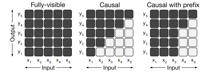
The different variations of masking in self-attention mechanism can be seen in the following figure:
-
Fully-visible:
This allows a self-attention mechanism to attend to any entry of the input when producing each entry of its output. -
Causal:
This allows a self-attention mechanism to attend to only previous tokens. So, when producing the $i^{\text{th}}$ entry of the output sequence, causal masking prevents the model from attending to the $j^{\text{th}}$ entry of the input sequence for $j > i$. This masking can be used as a language model (LM), i.e. a model trained solely for next-step prediction -
Causal with prefix:
This is a special case of the causal masking where a fully-visible masking will be used during the prefix portion of the sequence and causal masking for the rest.
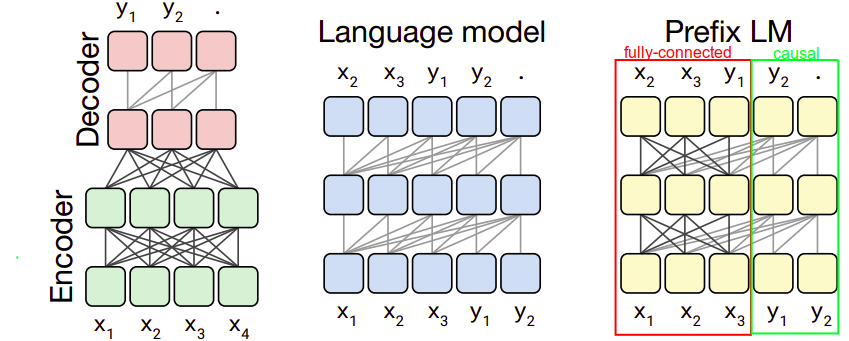
Using these three different masking techniques with the standard encoder-decoder transformer, we will get three different variations that will be used:
-
Encoder-decoder (left):
This is the same as the baseline; the encoder has no masking (fully-visible) while the decoder has a “causal masking”. -
Language Model (middle):
This architecture consists of a single Transformer layer stack and is fed the concatenation of the input and target using a causal mask throughout. -
Prefix LM (right):
This architecture is similar to language model with prefix-parameters (red rectangle) use fully-visible masking and the rest (green rectangle) use causal masking. This closely resembles BERT
Note:
The Prefix LM is similar to an encoder-decoder model with parameters shared across the encoder and decoder and with the encoder-decoder attention replaced with full attention across the input and target sequence.
Pre-training
In this paper, pre-training is done by running the model for $2^{19} = 524,288$ steps on C4 before fine-tuning. A maximum sequence length of $512$ is used and a batch size of $128$ sequences and they packed multiple sequences into one entry of the batch whenever possible. Roughly speaking, models in this paper are pre-trained on $2^{35} \approx 34B$ tokens which is considerably less than BERT ($137B\ $tokens) or RoBERTa ($2.2T$ tokens).
Note:
That $2^{35}$ tokens only covers a fraction of the entire C4 dataset which means they never repeated any data during pre-training.
Also, they used an “inverse square root” learning rate schedule: $\frac{1}{\sqrt{\max\left( n,k \right)}}$ where $n$ is the current training iteration and $k$ is the number of warm-up steps which was set to $10^{4}$. This sets a constant learning rate of $0.01$ for the first $10^{4}$ steps, then exponentially decays the learning rate until pre-training is over.
Since fine-tuning will be done on other languages other than English like (German, French, and Romanian), they classified the pages in C4 that are either German, or French, or Romanian. Then, they trained the SentencePiece model on a mixture of 10 parts of English C4 data with 1 part for each language forming a vocabulary of $32,000$ word-pieces.
Very Important Note:
Based on this vocabulary setup, T5 models can only process a predetermined, fixed set of languages which are English, German, French, and Romanian.
Objectives
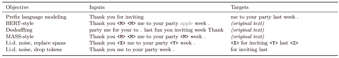
The choice of unsupervised objective is of central importance as it provides the mechanism through which the model gains general-purpose knowledge to apply to downstream tasks. All objectives mask one or multiple tokens from the input to produce a (corrupted) input that the model will learn to predict the target sequence with the maximum likelihood. The following table summarizes all pre-training objectives discussed in this paper and they are:
-
Prefix Language Modeling:
This technique splits a span of text into two components, one to use as inputs to the encoder and the other to use as a target sequence to be predicted by the decoder. -
BERT-style:
BERT-MLM objective takes a span of text and corrupts $15\%$ of the tokens. BERT had only an encoder without a decoder. So, in this encoder-decoder setup, they adapted MLM from BERT by simply using the entire uncorrupted sequence as the target. -
De-shuffling:
This approach takes a sequence of tokens, shuffles it, and then uses the original de-shuffled sequence as a target. -
MASS-style:
This approach masks a consecutive sequence of tokens in the input and passes it to the encoder, then use the uncorrupted sequence as the target. This looks like the Masked-Sequence objective discussed in MASS with a few changes. -
i.i.d. noise, replace spans:
This approach avoid predicting the whole uncorrupted text by masking a few tokens in the encoder. Then, the target sequence becomes the concatenation of the “corrupted” spans, each prefixed by the mask token used to replace it in the input. -
i.i.d. noise, drop tokens:
It’s the same as I.i.d. noise, replace spans but with dropping the corrupted tokens from the input sequence, then use these dropped tokens (in order) as the target.
Notes:
$\left\langle M \right\rangle$ denotes a shared mask token (with same ID) while $\left\langle X \right\rangle$, $\left\langle Y \right\rangle$, and $\left\langle Z \right\rangle$ denote sentinel tokens that are assigned unique token IDs.
The greyed-out word “apple” in the previous table shows that this token is a random token used as a replacement.
All objectives mentioned earlier except the prefix LM are called “denoising” objectives, since they add a noise to the input and the model has to de-noise it.
The replace spans approach later will be called “Span Corruption”.
The “i.i.d” written before the objective name of the last two objectives indicates that for each input token, a decision will be made to either corrupt the token or leave it as it is.
Fine-Tuning
All models in this paper were fine-tuned for $2^{18} = 262,144$ steps on all tasks. This value was chosen as a trade-off between the high-resource tasks (i.e. those with large data sets), which benefit from additional fine-tuning, and low-resource tasks (smaller data sets), which overfit quickly. Like pre-training, they used batches with $128$ length-$512$ sequences. And unlike pre-training, they used a constant learning rate of $0.001$.
They saved a checkpoint every $5,000$ steps and report results on the checkpoint that got the highest validation performance. For models fine-tuned on multiple tasks, they chose the best checkpoint for each task independently.
Benchmarks
They used a diverse set of benchmark (all sourced from TensorFlow datasets) that is able to measure the general language learning; these datasets are:
-
GLUE and SuperGLUE for text classification.
-
CNN/Daily Mail for abstractive summarization.
-
SQuAD for question answering.
-
WMT (English → German), (English → French), and (English → Romanian) for machine translation.
Results
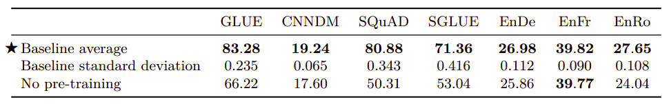
In this part, we are going to discuss all the experiments they tried in the paper and what we can learn from them. The results tables are all formatted so that each row corresponds to a particular experimental configuration with columns giving the scores for each benchmark. The baseline configuration is marked with ★. Any score that is within two standard deviation of the best score in a given experiment will be bold-faced. Also, all results are reported on the validation set of each benchmark dataset.
- Baseline (with/without pre-training):
The following table shows the average and standard deviation of the baseline model with and without pre-training for the same number of steps:
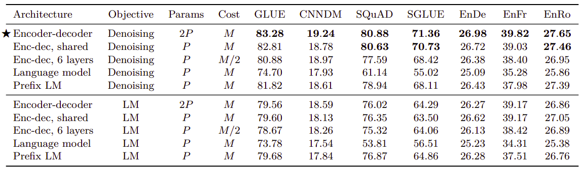
- Architectural Variants:
The following table shows the performance when trying different architectural variants pre-trained on a certain objective and fine-tuned on the benchmark. To provide a reasonable means of comparison, they referred to the number of layers in BERT~BASE~-sized layer stack as $L$ and the number of parameters as $P$ and the number of FLOPs (Floating-point Operations) required for an $L + L$-layer encoder-decoder model or $L$-layer decoder-only model as $M$.
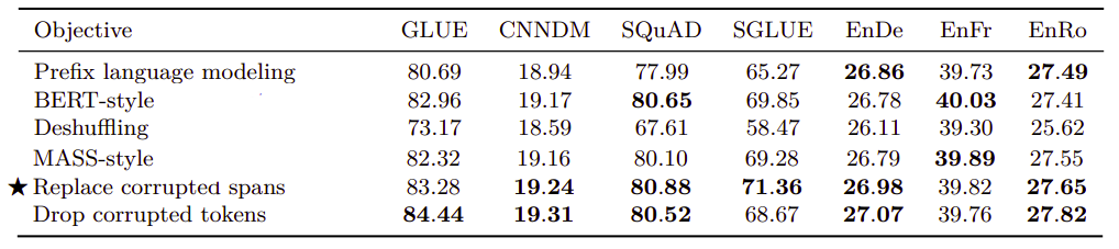
- Objective Functions:
The following table shows the performance of the baseline model using different objective functions; from the table we can see that all BERT-style variants (BERT-style + the last three) perform similarly.
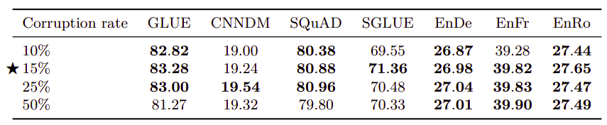
- BERT-style Corruption Rate:
As you remember, BERT-style corruption rate masks 15% of the input sequence; 80% with the $\left\langle M \right\rangle$ token; 10% with a random token and 10% with the original token. In the following table, they tried different corruption rate. From the table, we can see that the corruption rate had a limited effect on the model’s performance. The only exception is (50%), it results in a significant degradation of performance on GLUE and SQuAD.
- Span Length:
Span length is the number of consecutive tokens that will be masked when applying the denoising objective. Using a corruption rate of $15\%$ in all cases, the following table compares average span lengths of 2, 3, 5 and 10. The baseline (i.i.d) means that for each input token, we will have to make a decision whether to corrupt it or not. Again, this shows limited difference except with an average span length of 10 which slightly under-performs the other values in some cases.

-
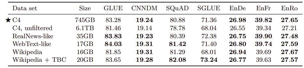
Pre-training datasets:
The following table measures the effect of different C4 filtration methods (first four entries) alongside with common pre-training datasets (last two) on downstream tasks performance:-
Unfiltered C4: ignoring all C4 filtration steps mentioned earlier except the one using the langdetect tool to extract English data.
-
RealNews-like: using standard filtration on C4 and to only include content from one of the domains used in the “RealNews” dataset.
-
WebText-like: using standard filtration on C4 and to only use content originated from a URL that appeared in the list prepared by the OpenWebText. This was relatively small (around 2GB). Therefore, they used 12 months (August 2018 to July 2019) from CommonCrawl instead of just one months as the original C4.
-
Wikipedia: using the English Wikipedia text data from TensorFlow Datasets, which omits any markup or reference sections from the articles.
-
Wikipedia + Toronto Books Corpus: A drawback of using pre-training data from Wikipedia is that it represents only one possible domain of natural text (encyclopedia articles). To mitigate this, they combined the Wikipedia data with the Toronto Books Corpus (TBC). TBC contains text extracted from eBooks, which represents a different domain of natural language. This is the same pre-training data used with BERT.
-
- Pre-training data size:
The following table measures the effect of limited unlabeled dataset sizes. These results were obtained by truncating the first $2^{29}$, $2^{27}$, $2^{25}$, and $2^{23}$ tokens of the C4 dataset. Knowing that all models in this paper were trained using $2^{35}$ tokens, these data sizes had to be repeated to match that. From the table, the performance degrades as the data set size shrinks which is totally expected:

- Alternative fine-tuning Methods:
The following table compares different alternative fine-tuning methods that only update a subset of the model’s parameters. For adapter layers, $d$ refers to the inner dimensionality of the adapters. As we can see, lower-resource tasks like SQuAD work well with a small value of $d$ whereas higher resource tasks require a large dimensionality to achieve reasonable performance.

Note:
The past experiment suggests that adapter layers could be a promising technique for fine-tuning on fewer parameters as long as the dimensionality is scaled appropriately to the task size.
Multi-task Learning
So far, we have been pre-training our model on a single unsupervised learning task before fine-tuning it individually on each downstream task. An alternative approach, called “multitask learning”, is to train the model on multiple tasks at once. In this paper, they relaxed that goal somewhat and instead investigated methods for training on multiple tasks at once in order to eventually produce separate parameter settings that perform well on each individual task which makes it comparable to the pre-train-then-fine-tune approach.
Multi-task learning is performed on the same datasets as the fine-tuning An extremely important factor in multi-task learning is how much data from each task the model should be trained on. In this paper, they have tried three different mixing methods to make sure each task gets enough data:
-
Equal mixing:
In this case, each example in each batch is sampled uniformly at random from one of the datasets. -
Example-proportional Mixing:
If the number of examples in each of the $N$ task’s data sets is $e_{n}$ where $n \in \left\{ 1,\ …N \right\}$, then the probability of sampling an example from the $m^{\text{th}}$ task during training is $r_{m} = \frac{\min\left( e_{n},\ K \right)}{\sum_{i = 1}^{N}{\min\left( e_{i},\ K \right)}}$ where $K$ is the artificial data set size limit. -
Temperature-scaled mixing:
Temperature up-samples the relatively low-resource tasks. This is done by raising each task’s mixing rate $r_{m}$ to the power of $\frac{1}{T}$.
To compare these mixing strategies on equal footing with the pre-train-then-fine-tune results, they trained multi-task models for the same total number of steps: $2^{19} + 2^{18} = 786,432$. The results are shown in the following table:
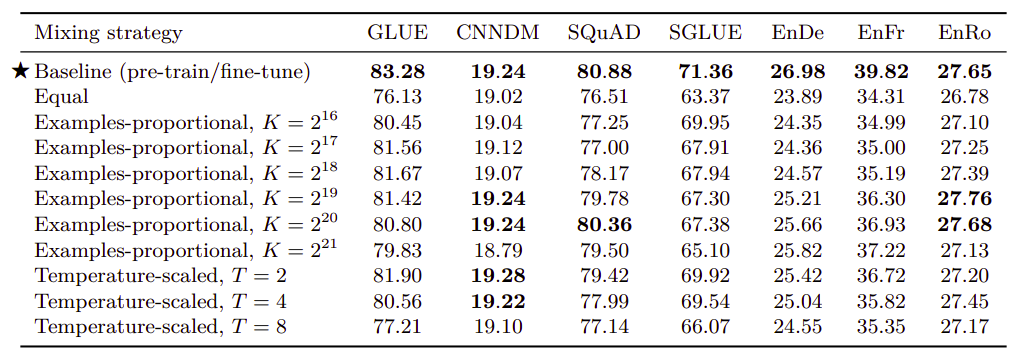
From the table, we can find out that multi-task training under-performs pre-training followed by fine-tuning on most tasks. The “equal” mixing strategy in particular results in dramatically degraded performance.
Since they relaxed the multi-task learning to make it look similar to the pre-train-then-fine-tune-approach, they decided to combine fine-tuning with multi-task learning once and combine multi-task learning with pre-training another time. The following table shows that the pre-train and then fine-tune technique is still better:

All multi-task learning performed in the previous table were mixed using examples-proportional method (with $K = 2^{19}$). Leave-one-out multi-task training was done by pre-training the model on all tasks except one and then fine-tune it on the task that was left out during pre-training.
Scaling
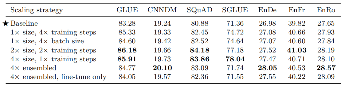
In deep learning, there is an argument that says that scaling up models produces improved performance. However, there are a variety of possible ways to scale (to make model bigger) like using more parameters, training the model for more steps, and ensembling. In the paper, they compared these different approaches with the baseline model.
To increase the number of parameters, they experimented with the BERT~LARGE~ setup with $d_{\text{ff}} = 4096$, $d_{\text{model}} = 1024$, $d_{\text{kv}} = 64$, and $16$-head attention mechanism and $16$-layers encoder and $16$-layers decoder. This setup produces twice ($2 \times$) the number of parameters as the baseline model. Using $32$-layers encoder and $32$-layers decoder will produce roughly four times ($4 \times$) the number of parameters as the baseline model. Also, created an ensemble model by training the baseline 4 different times and averaging their results.
The performance achieved after applying these various scaling methods is shown in the following table which shows that increasing the model size resulted in an additional bump in performance compared to solely increasing the training time or batch size:
Important Notes:
Different scaling methods have different trade-offs that are separate from their performance. For example, using a larger model can make downstream fine-tuning and inference more expensive. In contrast, the cost of pre-training a small model for longer is effectively amortized if it is applied to many downstream tasks.
Ensembling $N$ separate models has a similar cost to using a model that has an $N \times$ higher computational cost.