Transformers
Transformer architecture is a novel architecture for encoder-decoder paradigm created in an attempt to combine all good things from Seq2Seq architecture and ConvS2S with attention mechanisms. Transformer was proposed by a team from Google Research and Google Brain in 2017 and published in a paper under the name: “Attention is all you need”. The official code for this paper can be found on the Tensor2Tensor official GitHub repository: tensor2tensor.
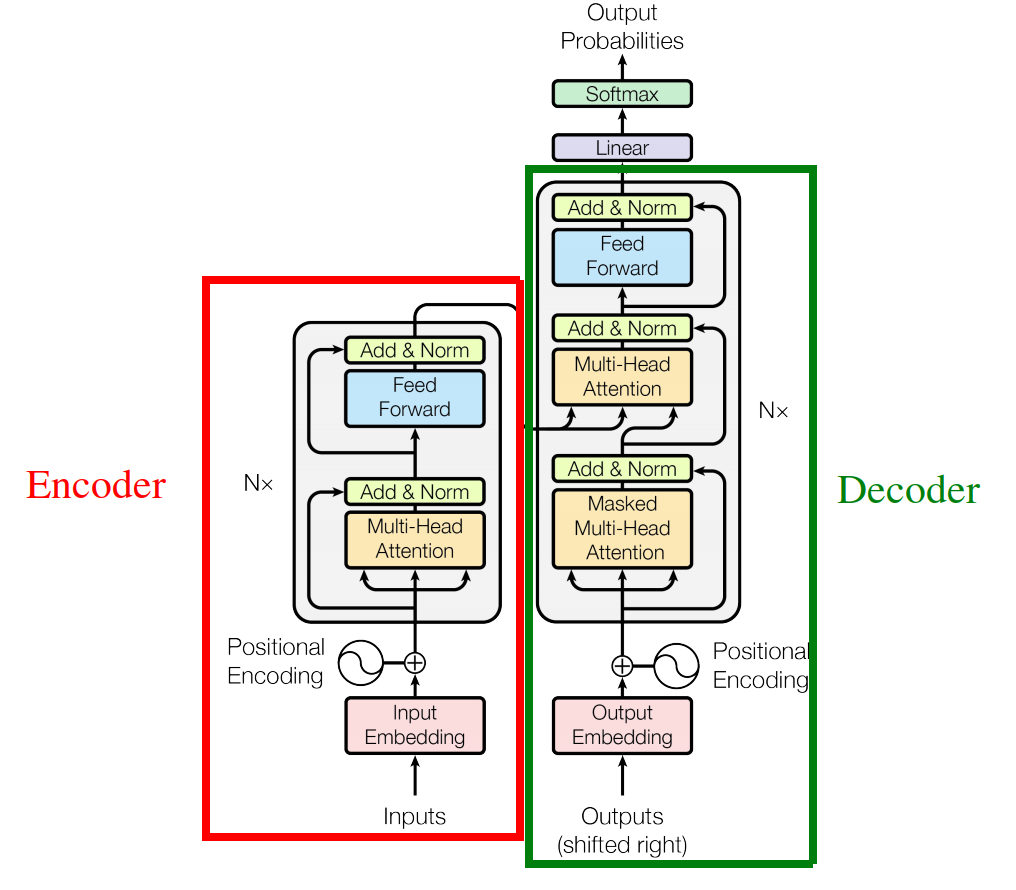
Transformer architecture deals with the input text data in an encoder-decoder manner the same as Seq2Seq and tries to parallelize the input data the same as ConvS2S. In this paper, the Transformer architecture consists of six layers of encoder and six layers of decoder as shown in the following figure:
Architecture
Most competitive machine translation models have an encoder-decoder structure where the encoder maps an input sequence of symbol representations $X = \left( x_{1},\ …x_{n} \right)$ to a sequence of continuous representations $Z = \left( z_{1},\ …z_{n} \right)$. Given $Z$, the decoder then generates an output sequence $Y = \left( y_{1},\ …y_{m} \right)$ of symbols in an autoregressive manner (one token at a time).
The most critical and influential part of the Transformer is the attention mechanism which takes a quadratic time and space over the input sequence which makes training Transformer takes longer time that Seq2Seq and ConvS2S models. In this transformer architecture, there are three different attention mechanisms used:
-
Attention between the input tokens (self-attention).
-
Attention between the output tokens (self-attention).
-
Attention between the input and the output tokens
Note:
The attention between the input (or output) tokens is called self-attention because the attention is between the same parameters.
Padding
To be able to parallelize sentences with different lengths in transformer, we need to define a value that represents the maximum length (MAX_LENGTH) found in our training data. And all sentences whose length is less than MAX_LENGTH should be padded using a PAD vector.
So, in the following image we have a mini-batch of three sentences where the longest one is seven-tokens long. And the MAX_LENGTH is nine. In practice, PAD is the $0^{th}$ index of the embedding matrix which means it will be learnable vector. It’s learnable for convenience not because we need it to be. Also, the PAD vector should be ignored when computing the loss.
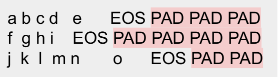
Note: In fairseq framework, padding is done randomly at either the beginning of the sentence or at the end. Also, the pad token
<p>has an index of1while index0is reserved for the beginning of the sentence token<s>.
Encoder
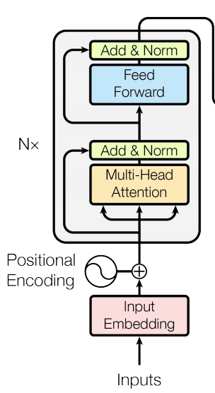
We are going to focus on the encoder part of the transformer architecture which consists of different modules:
-
Embedding: where we map words into vectors representing their meaning such that similar words will have similar vectors. The embedding matrix have a size of $\mathbb{R}^{n \times d_m}$ where $n$ is the input length and $d$ is the embedding dimension.
-
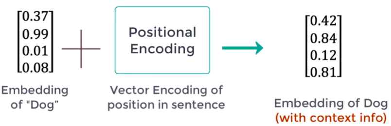
Positional Encoding: Word meaning differs based on its position in the sentence. A positional vector is a vector of the same size as the embedding vector that gives context based on word-position in a sentence. This can be done by applying following equation:
Where $pos$ is the word position/index (starting from zero). $i$ is the $i^{th}$ value of the word embedding and $d_m$ is the size of the word embedding. So, if $i$ is even, then we are going to apply the first equation; and if $i$ is odd, then we are going to apply the second equation. After getting the positional vectors, we add them to the original embedding vector to get context vector:
I know these functions don’t make sense and the original paper says the following:
“We tried to encode position into word embedding using sinusoidal functions and using learned positional embeddings, and we found that the two versions produced nearly identical results.”
But in case you wanted to dig deeper in this part, check this YouTube video. It’s a good start. Also, look into this article.
- Single-Head Self-Attention:
Self-attention allows the encoder to associate each input word to other words in the input. To achieve self-attention, we feed the embedded input $X \in \mathbb{R}^{n \times d_{m}}$ into three different linear fully-connected layers $W^{Q},W^{K} \in \mathbb{R}^{d_{m} \times d_{k}},\ W^{V} \in \mathbb{R}^{d_{m} \times d_{v}}$ producing three different matrices respectively; which are query $Q \in \mathbb{R}^{n \times d_{k}}$, key $K \in \mathbb{R}^{n \times d_{k}}$, and value $V \in \mathbb{R}^{n \times d_{v}}$.
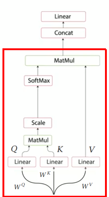
Now, the attention mechanism will attend the resulting three matrices via the following equation:
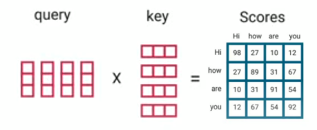
\[\text{Attention}\left( Q,\ K,\ V \right) = softmax\left( \frac{QK^{T}}{\sqrt{d_{k}}} \right)V\]So, we are going to perform a dot product of Q and K to get a score matrix that scores the relation between each word in the input and the other words in the input as well.
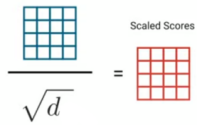
Then, these scores are getting scaled down by dividing over the square root of the dimension of query and key (which is $d$) to allow more stable gradients as the dot product could lead to exploding values:
Then, we are going to perform a Softmax over these down-scaled scores to get the probability distribution which is called the attention weights:
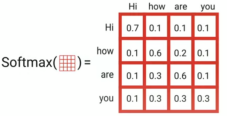
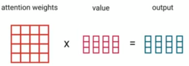
Finally, we are going to perform a dot product between the attention weights and the values V to get an output vector. The higher the attention weight is, the higher it contributes to the output vector.
Note: The name of these three vectors comes from retrieval systems. So, when you type a query on Google to search for, this query will be mapped to a set of results keys to score each result. And the highest results will be the values you were looking for.
- Multi-Head Self-Attention:
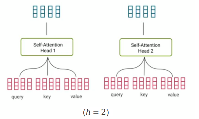
A multi-head self-attention is just performing the single-head self-attention $h$ times and concatenating the output matrices together before applying a linear layer $W^{O} \in \mathbb{R}^{h d_v \times d_m}$ as shown in the following formula:
In theory, this will make each head learn something different about the input. After concatenation, we apply a linear fully-connected layer to match dimensions for the residual connection. The following image shows the multi-head attention of just two heads $h=2$:
- Residual Connection & Normalization: After the multi-head self-attention, the positional input embedding is added to the output vectors. This is known as a “residual connection” which is mainly used to prevent gradient from vanishing. After that, a layer normalization is applied:
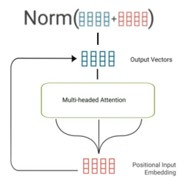
Then, we apply a batch or layer normalization. The difference is pretty subtle where the batch normalization normalizes over all data in the batch and the layer normalization normalizes over all weights in the layer.
- Feed-forward: Now, the normalization output gets fed to the feed-forward network for further processing. The feed-forward network is just a couple of linear layers with a $\text{ReLU}$ activation function in between. The dimension of the feed-forward network is defined by the $d_{\text{ff}}$ parameter where $W_1 \in \mathbb{R}^{d_{m} \times d_{ff}}, W_2 \in \mathbb{R}^{d_{ff} \times d_{m}}$ are the learnable weights and $b_1 \in \mathbb{R}^{d_{ff}}, b_2 \in \mathbb{R}^{d_{m}}$ are the learnable biases.
Decoder
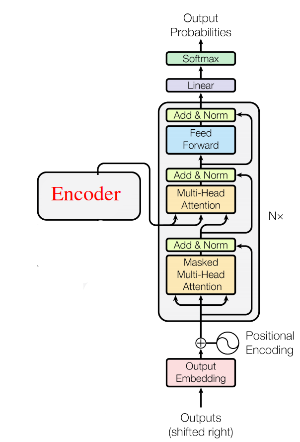
In this part, we are going to focus on the decoder part of the transformer architecture. As we can see, it’s the same components as the encoder except for two things:
-
Shifted-right inputs: Input (sentence in another language) is shifted right by one word while training because we want to make sure the encoder was able to get this word before updating its value.
-
Masked Multi-Head self-Attention: The masked multi-head is a little bit different than the multi-head self-attention one. As the masked one will only be able to access the previous words not the following one. In order to solve that, we are going to create look-ahead mask matrix that masks any further values with -inf.
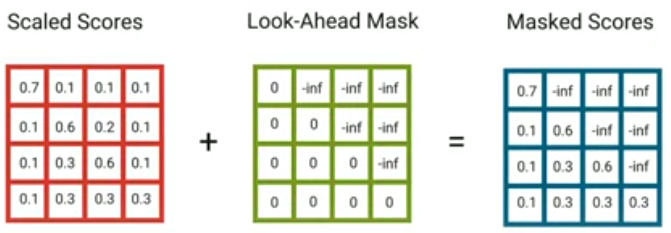
We are using -inf as a small numbers that will be zero when applying the Softmax.
- Multi-head Attention #2: The query and key of this block will come from the encoder output and the values will be the output of the masked multi-head block.
Training
Before training, sentences were encoded using byte-pair encoding with a shared source-target vocabulary of about $37,000$ tokens for WMT English-German and 32,000 for English-French.
For training, each training batch contained approximately $25,000$ tokens. They used Adam optimizer with $\beta_{1} = 0.9,\ \beta_{2} = 0.98$ and $\epsilon = 10^{- 9}$. Learning rate was varied over the course of training, according to the following formula:
\[lr = d_{\text{model}}^{- 0.5}.\min\left( {step\_ num}^{- 0.5},\ step\_ num*{warmup\_ steps}^{- 1.5} \right)\]This corresponds to increasing the learning rate linearly for the first $\text{warmup_steps}$ training steps, and decreasing it thereafter proportionally to the inverse square root of the $\text{step_num}$. They used $\text{warmup_steps} = 4000$.
For regularization, they used dropout to the output of each sub-layer, before it is added to the sub-layer input and normalized. In addition, they applied dropout to the sums of the embeddings and the positional encodings in both the encoder and decoder stacks. Also, label smoothing $\epsilon_{l_{s}} = 0.1$ was used.
There were two variants of the Transformer configurations found in the paper, Transformer-base and Transformer-big configurations which can be summarized in the following table:
| $$N$$ | $$d_{m}$$ | $$d_{\text{ff}}$$ | $$h$$ | $$d_{k}$$ | $$d_{v}$$ | $$P_{\text{dropout}}$$ | $$\epsilon_{l_{s}}$$ | # parameters | train steps | |
|---|---|---|---|---|---|---|---|---|---|---|
| Base | 6 | 512 | 2048 | 8 | 64 | 64 | 0.1 | 0.1 | 65 M | 100k |
| Large | 6 | 1024 | 4096 | 16 | 64 | 64 | 0.3 | 0.1 | 213 M | 300k |
For decoding, they used beam search with a $\text{beam size} = 4$ and length penalty $\alpha = 0.6$.
The following table shows that the big transformer model achieves state-of-the-art performance on the WMT 2014 English-German translation task and English-French translation:
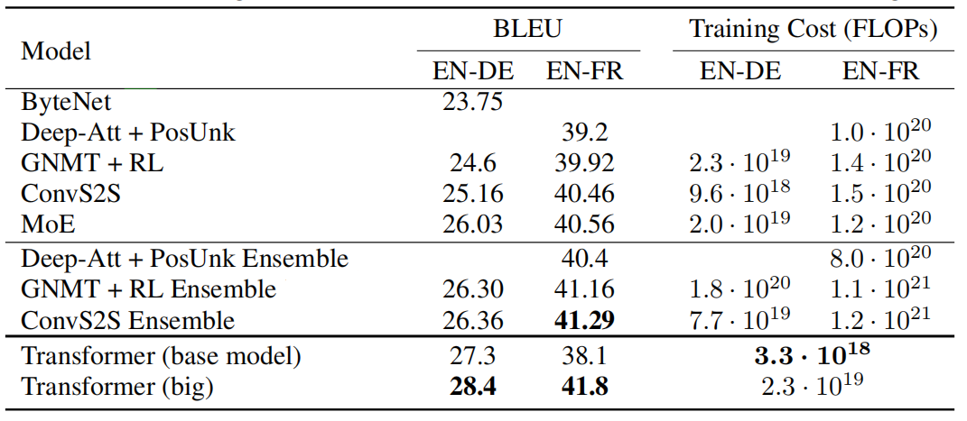
The base models score was obtained by averaging the last 5 checkpoints, which were written at 10-minute intervals. For the big models, the last 20 checkpoints were averaged.
Note:
For the English-French dataset, the big transformer used $P_{\text{dropout}} = 0.1$, instead of $P_{\text{dropout}} = 0.3$.
Layer Normalization
Normalization is an important part of the Transformer architecture as it improves the performance and avoids the overfitting. Here, we are going to discuss the different layer normalization techniques that can be used based as suggested by this paper: Transformers without Tears: Improving the Normalization of Self-Attention The official code for this paper can be found in this GitHub repository: transformers_without_tears.
This paper compares between two different orders of layer normalization in the Transformer architecture:
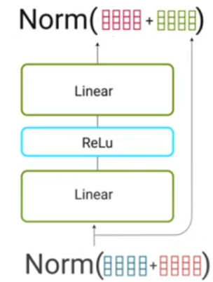
- Post-Norm:
Post-normalization is the default type of normalization used in the standard Transformer architecture. It’s called that because it occurs after the residual addition:
- Pre-Norm:
Pre-normalization is applied immediately before the sublayer. Pre-Norm enables warmup-free training providing greater stability and doesn’t get affected by the weight initialization unlike Post-Norm:
Very Important Note:
In the paper, they found out that post-normalization works best with high-resource languages while pre-normalization works best with low-resource languages.
Also, in the paper, they proposed an alternative to the layer normalization:
- Scale-Norm: Scale-Norm is an alternative for layer normalization. As we can see from the following equation, Scale-Norm replaced the two learnable parameters $\gamma,\ \beta$ in layer normalization with one global learned scalar $g$:
- Scale-Norm + Fix-Norm: Fix-Norm is applied to the word embeddings. It looks exactly like Scale-Norm with only one global learnable scalar g, so we can apply both of them jointly like so:
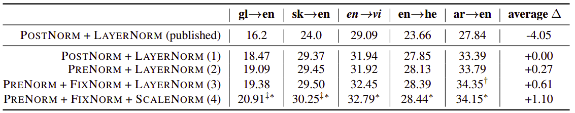
And the following are the results published in the paper on various machine translation directions:
LayerDrop
LayerDrop is a novel regularization method for Transformers used to prevent them from overfitting. This method was proposed by Facebook AI in 2019 and published in this paper: Reducing Transformer Depth On Demand With Structured Dropout. The official code for this paper can be found in the official Fairseq GitHub repository: fairseq/layerdrop.
Deep Networks with Stochastic Depth paper has shown that dropping layers during training can regularize and reduce the training time of very deep convolutional networks. And this is the core idea of LayerDrop where entire layers are randomly dropped at training time which regularizes very deep Transformers and stabilizes their training, leading to better performance.
The following figure shows a comparison of a 9-layer transformer trained with LayerDrop (right) and 3 transformers of different sizes (left). As we can see, the different pruned version of the transformer on the right obtained better results than the same sized transformers trained from scratch:
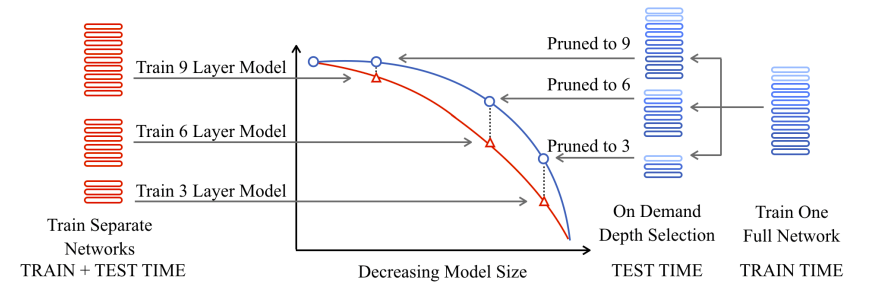
Which shows that LayerDrop also acts like a distillation technique that can lead to small and efficient transformers of any depth which can be extracted automatically at test time from a single large pre-trained model, without the need for finetuning.
LayerDrop does not explicitly provide a way to select which group of layers will be dropped. So, the publishers considered several different pruning strategies:
-
Every Other: A straightforward strategy is to simply drop every other layer. Pruning with a drop rate $p$ means dropping the layers at a depth $d$ such that $d \equiv 0\left( \text{mod}\left\lfloor \frac{1}{p} \right\rfloor \right)$. This strategy is intuitive and leads to balanced networks.
-
Search on Valid: Another possibility is to compute various combinations of layers to form shallower networks using the validation set, then select the best performing for test. This is straightforward but computationally intensive and can lead to overfitting on validation.
-
Data Driven Pruning: Another approach is to learn the drop rate of each layer. Given a target drop rate $p$, we learn an individual drop rate $p_{d}$ for the layer at depth $d$ such that the average rate over layers is equal to $p$.
The “Every Other” works the best with the following drop rate $p$ where $N$ is the number of layers, $r$ is the target pruned size:
Note:
In the paper, they used a LayerDrop rate of $p = 0.2$ for all their experiments. However, they recommend using $p = 0.5$ to obtain very small models at inference time.
DropHead
DropHead is another novel regularization method for Transformers used to prevent overfitting. This method was proposed by Microsoft Research Asia in 2020 and published in this paper: Scheduled DropHead: A Regularization Method for Transformer Models. There is unofficial implementation for this paper, it can be found in this GitHub repository: drophead-pytorch.
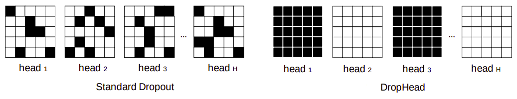
In the core, DropHead drops entire attention heads during training to prevent the multi-head attention model from being dominated by a small portion of attention heads which can help reduce the risk of overfitting and allow the models to better benefit from the multi-head attention. The following figure shows the difference between dropout (left) and DropHead (right):
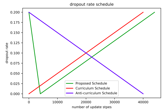
In the paper, they proposed a specific dropout rate scheduler for the DropHead mechanism, which looks like a V-shaped curve (green curve below): It applies a relatively high dropout rate of $p_{\text{start}}$ and linearly decrease it to $0$ during the early stage of training, which is empirically chosen to be the same training steps for learning rate warmup. Afterwards, it linearly increases the dropout rate to $p_{\text{end}}$. To avoid introducing additional hyper-parameters, they decided to set $p_{\text{start}} = p_{\text{end}}$.