NAT: Non-Autoregressive Transformer
NAT, stands for “Non-Autoregressive Translation”, is an NMT model that avoids the autoregressive property of the decoding and produces its outputs in parallel. NAT was created by Salesforce in 2017 and published in their paper: “Non-Autoregressive Neural Machine Translation”. The official code for this paper can be found on the official Salesforce GitHub repository: nonauto-nmt.
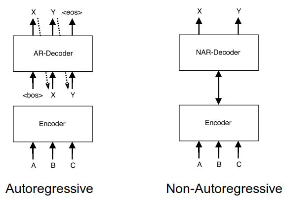
Before getting into Non-Autoregressive model, let’s first recap what is an Autoregressive model. Given a source sentence $X = \left( x_{1},\ …x_{m} \right)$, an Autoregressive model factors the distribution over possible output sentences $Y = \left( y_{1},\ …y_{n} \right)$ into a chain of conditional probabilities with a an auto-regressive (left-to-right) manner as shown below:
\[p\left( Y \middle| X;\theta \right) = \prod_{t = 1}^{n}{p\left( y_{t} \middle| y_{0:t - 1},\ x_{1:m};\ \theta \right)}\]Where the special tokens $y_{0} = \left\langle \text{bos} \right\rangle$ and $y_{n + 1} = \left\langle \text{eos} \right\rangle$ are used to represent the beginning and end of all target sentences. These conditional probabilities are parameterized using a neural network $\theta$.
NAT Architecture
The autoregressive model corresponds to the word-by-word nature of human language production and effectively captures the distribution of real translations. That’s why they achieve state-of-the-art performance on large-scale corpora. But there are also drawbacks such as individual steps of the decoder must be run sequentially rather than in parallel which takes longer. The NAT model proposed in this paper tries to solve that problem:
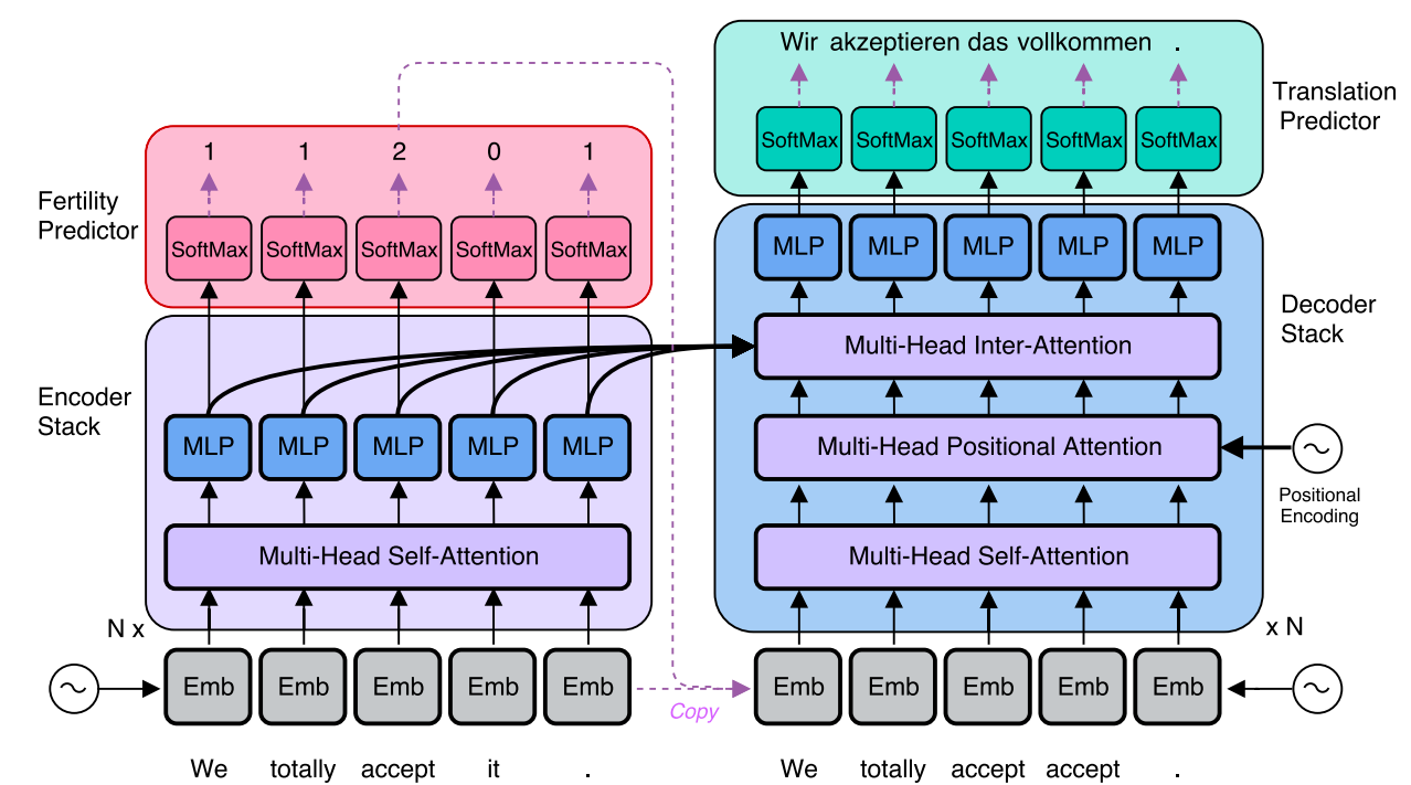
The NAT model, as shown in the following figure, is composed of the following four modules: Encoder stack, Decoder stack , a newly added fertility predictor added at the end of the encoder stack, and a translation predictor added at the end of the decoder stack.
Encoder Stack
The encoder stays unchanged from the original Transformer network ☺.
Decoder Stack
To be able to parallelize the decoding process, the NAT needs to know how long the target sentence will be. And since the target sentence length is different but not that far from the source sentence, they initialized the decoding process using copied source inputs from the encoder side based on the word’s “fertility”.
Since we are processing the output as a whole, we no longer need the masking before the self-attention. Instead, they only masked out each query position only from attending to itself, which they found to improve decoder performance relative to unmasked/standard self-attention.
Also, they added a new block called “Multi-head Positional Attention” in each decoder layer, which is a multi-head attention module with the same general attention mechanism used in other parts of the Transformer network:
\[\text{Attention}\left( Q,K,\ V \right) = \text{softmax}\left( \frac{QK^{T}}{\sqrt{d_{\text{model}}}} \right)\text{.V}\]This incorporates positional information directly into the attention process and provides a stronger positional signal than the embedding layer alone.
Fertility Predictor
Words’ fertility are integers for each word in the source sentence that correspond to the number of words in the target sentence that can be aligned to that source word if a hard alignment algorithm was used (like IBM Models for example).
Using the fertility predictor and given a source sentence $X = \left( x_{1},\ …x_{m} \right)$, the conditional probability over the possible output sentence $Y = \left( y_{1},\ …y_{n} \right)$ is:
\[p\left( Y \middle| X;\theta \right) = \sum_{f_{1},\ ...f_{m} \in \mathcal{F}}^{}\left( \prod_{t = 1}^{m}{p_{F}\left( f_{t} \middle| x_{1:m};\ \theta \right)}.\prod_{t = 1}^{n}{p\left( y_{t} \middle| x_{1}\left\{ f_{1} \right\},\ ...x_{m}\left\{ f_{m} \right\};\ \theta \right)} \right)\]Where:
- $\mathcal{F} \in \left( f_{1},\ …f_{m} \right)$ is the set of all fertility sequences, one fertility value per source token. Knowing that the sum of all fertility values is the length of the target sentence:
-
$p_{F}\left( f_{t} \middle| x_{1:m};\ \theta \right)$ is the fertility prediction model which is a one-layer neural network with a softmax classifier ($L = 50$ in these experiments) on top of the output of the last encoder layer. This models the way that fertility values are a property of each input word but depend on information and context from the entire sentence.
-
$x\left\{ f \right\}$ denotes the source token $x$ repeated $f$ times.
Translation Predictor
At inference time, the model can identify the translation with the highest conditional probability by marginalizing over all possible latent fertility sequences. In other words, the optimal output translation sequence given a source sentence $x$ and an optimal sequence of fertility values $\widehat{f}$ is:
\[\widehat{Y} = G\left( x_{1:m},\ {\widehat{f}}_{1:m};\theta \right)\]As seen from the previous equation, finding an optimal output translation sequence heavily depends on the fertility values. To search over the whole fertility space is a big task. So, they proposed three heuristic decoding algorithms to reduce the search space of the NAT model given the fertility distribution $p_{F}$:
- Argmax Decoding:
The optimal sequence of fertility value is the highest-probability fertility for each input word:
- Average Decoding:
The optimal sequence of fertility value is the the expectation of its corresponding softmax distribution ($L = 50$ in these experiments):
- Noisy parallel decoding (NPD):
A more accurate approximation of the true optimum of the target distribution is to draw samples from the fertility space and compute the best translation for each fertility sequence. We can then use the autoregressive teacher to identify the best overall translation:
Loss Function
Given a source sentence $X = \left{ x_{1},\ …x_{m} \right}$, a target sequence $Y = \left{ y_{1},\ …y_{n} \right}$ and a fertility values $f_{1:m}$, the loss function of the NAT model $\mathcal{L}$ can be described below:
\[\mathcal{L} = log\sum_{f_{1:m} \in \mathcal{F}}^{}{p_{F}\left( f_{1:m} \middle| x_{1:m};\ \theta \right)\text{.p}\left( y_{1:n} \middle| x_{1:m};\theta \right)}\]The resulting loss function allows us to train the entire model in a supervised fashion, using the inferred fertilities to simultaneously train the translation model $p$ and supervise the fertility neural network model $p_{F}$.
Note:
There are two possible options that can be used as labels for the the fertility network. The first is an external aligner, which produces a deterministic integer fertilities for each (source, target) pair in a training corpus. The second option is the attention weights used in an autoregressive teacher model.
After training the NAT model to convergence, they proposed a fine-tuning step where they freeze a trained autoregressive teacher model while train the NAT model on its soft labels. This introduced an additional loss term consisting of the reverse K-L divergence with the teacher output distribution:
\[\mathcal{L}_{\text{RKL}}\left( f_{1:m};\ \theta \right) = \sum_{t = 1}^{n}{\sum_{y_{t}}^{}\left\lbrack \text{log\ }p_{\text{AR}}\left( y_{t} \middle| {\widehat{y}}_{1:t},\ x_{1:m} \right).p_{\text{NA}}\left( y_{t} \middle| x_{1:m},\ f_{1:m};\theta \right) \right\rbrack}\]Where $p_{\text{AR}}$ is the probability distribution of the autoregressive teacher model, while $p_{\text{NA}}$ is the probability distribution of the NAT model. ${\widehat{y}}{1:t}$ is the optimal output sequence which equals to $G\left( x{1:m},\ f_{1:m};\theta \right)$. Such a loss is more favorable towards highly peaked student output distributions than a standard cross-entropy error would be.
Then they trained the whole model jointly with a weighted sum ($\lambda = 0.25$) of the original distillation loss and two such terms, one an expectation over the predicted fertility distribution, normalized with a baseline, and the other based on the external fertility inference model:
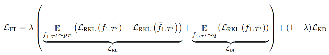
Where ${\overline{f}}{1:m}$ is the average fertility computed by the average decoding discussed before. The gradient with respect to the non-differentiable $\mathcal{L}{\text{RL}}$ term can be estimated with REINFORCE, while term $\mathcal{L}_{\text{BP}}$ can be trained using ordinary back-propagation
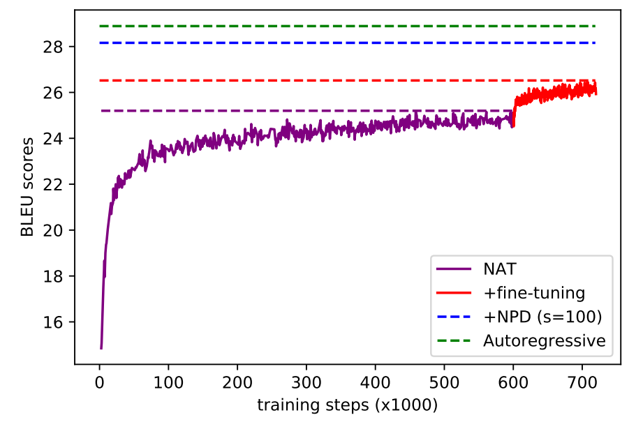
As seen from the below figure, using fine-tuning with a teacher model really helps improving the NAT model’s performance:
Results
Experiments were run on three widely used public machine translation corpora: IWSLT16 En-De, WMT14 En-De, and WMT16 En-Ro. All the data are tokenized using byte-pair encoding (BPE). For WMT datasets, BPE vocabulary were shared; for IWSLT, they used separate vocabulary. Additionally, they shared encoder and decoder word embeddings only in WMT experiments.
NAT model was initialized using the teacher model. The teacher model is a standard Transformer architecture with base configurations on the WMT dataset and smaller set of hyper-parameters when trained on IWSLT dataset since it’s smaller than WMT. The two sets of configuration can be seen below:
| $$N$$ | $$d_{m}$$ | $$d_{\text{ff}}$$ | $$h$$ | $$\epsilon_{l_{s}}$$ | Warmup steps | |
|---|---|---|---|---|---|---|
| WMT | 6 | 512 | 2048 | 8 | 0 | 10k |
| IWSLT | 5 | 287 | 507 | 8 | 0 | 746 |
The following table shows the BLEU scores on official test sets (newstest2014 for WMT En-De and newstest2016 for WMT En-Ro) and the development set for IWSLT. The NAT models without NPD use argmax decoding and latency is computed as the time to decode a single sentence without mini-batching, averaged over the whole test set:

As seen from the previous table, the NAT performs between 2-5 BLEU points worse than its autoregressive teacher across all three datasets.
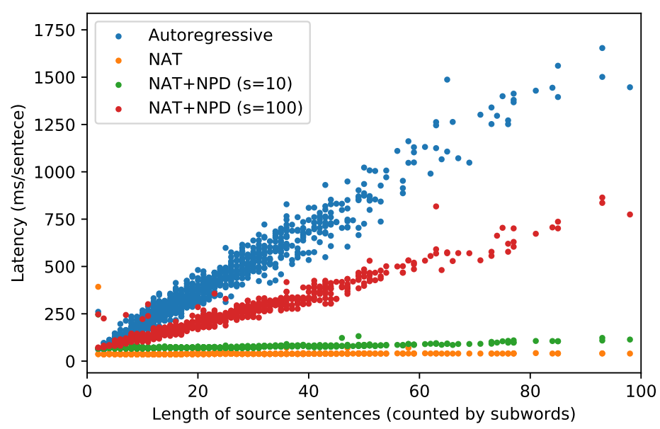
The translation latency, computed as the time to decode a single sentence without mini-batching, for each sentence in the IWSLT development set as a function of its length. The autoregressive model has latency linear in the decoding length, while the latency of the NAT is nearly constant for typical lengths:
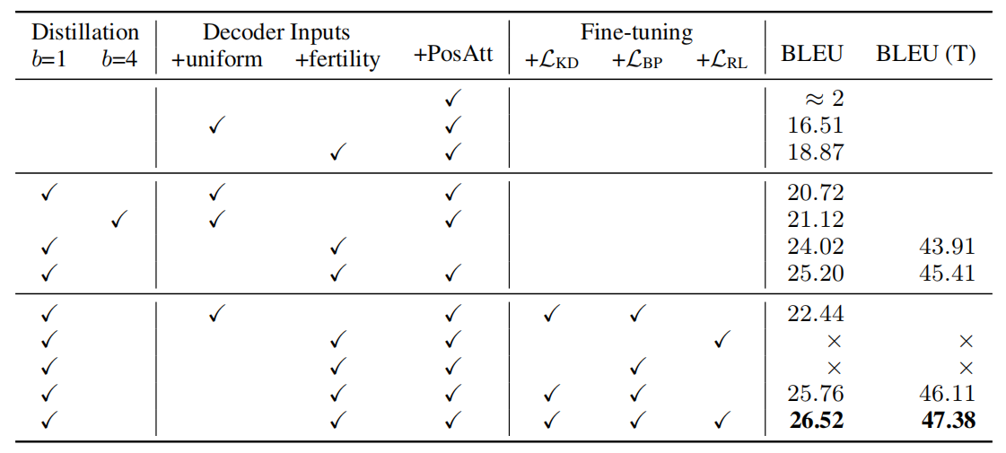
They also conducted an extensive ablation study with the proposed NAT on the IWSLT dataset. First, they noted that the model fails to train when provided with only positional embeddings as input to the decoder. Second, they found out using teacher model really helps. Third, the fertility-based copying improves performance by four BLEU points when using ground-truth training or two when using distillation.