Scaling Transformer

Scaling model sizes, datasets and the total computation budget has been identified as a reliable approach to improve generalization performance on several machine learning tasks. Here, we are going to discuss a paper called “Scaling Laws for Neural Machine Translation” published by Google Research in 2021 where the researchers study the effect of scaling the transformer depths on the performance.

Experiments

All experiments in this paper were performed using a series of Transformer networks where the model dimension to $1024$, feed-forward layer dimension to $8192$, number of attention heads to $16$, attention hidden dimension to $1024$, and varying layers as shown in the following figure knowing that the baseline is a 12-layer encoder 12-layer decoder Transformer model:

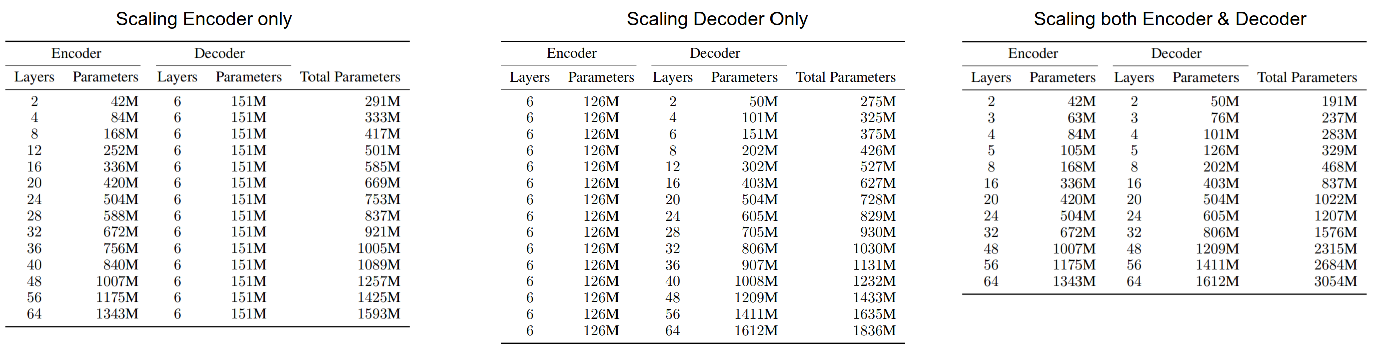
All models were trained with a cross-entropy loss and Adafactor optimizer. All models were trained for $500k$ training steps with a fixed batch-size of $500k$ tokens. All models were regularized using a dropout rate of $0.1$, label smoothing of $0.1$, and a gradient clipping of $10$ to improve the training stability.

Training Data

All results -in this paper- were reported on two language pairs, (English→German) and (German→English) using an in-house web-crawled dataset with around 2.2 billion sentence pairs for both translation directions. A sentence-piece vocabulary of size $32k$ was used for training all models. This dataset provides a large enough training set to ensure the dataset size is not a bottleneck in the model performance.

Evaluation Data

To evaluate these models, they used a variety of test sets covering different domains such as Web-Domain, News-Domain, Wikipedia, and Patents. The news-domain test sets come from the WMT2019 evaluation campaign (newstest2019) while the other test sets are internal test sets.

Throughout the paper, they refer to a certain data as either “source-original” or “target-original”, here is the difference:

• Source-original: means that the source sentences have been crawled from the web while the reference translations were generated later by professional translators.

• Target-original: means that the target sentences have been crawled from the web while the reference translations were generated later by professional translators.

Scaling Effect on Loss

In the paper, the researchers were able to find a formula that could capture the effect of scaling the encoder/decoder layers on the performance of a certain test set. Given the English→German web-domain test set, they trained multiple models with different encoder/decoder layers and measured the perplexity of each model on the test set. The following graph shows the performance of the encoder-scaling and decoder-scaling on source-original (left) and target-original (right):

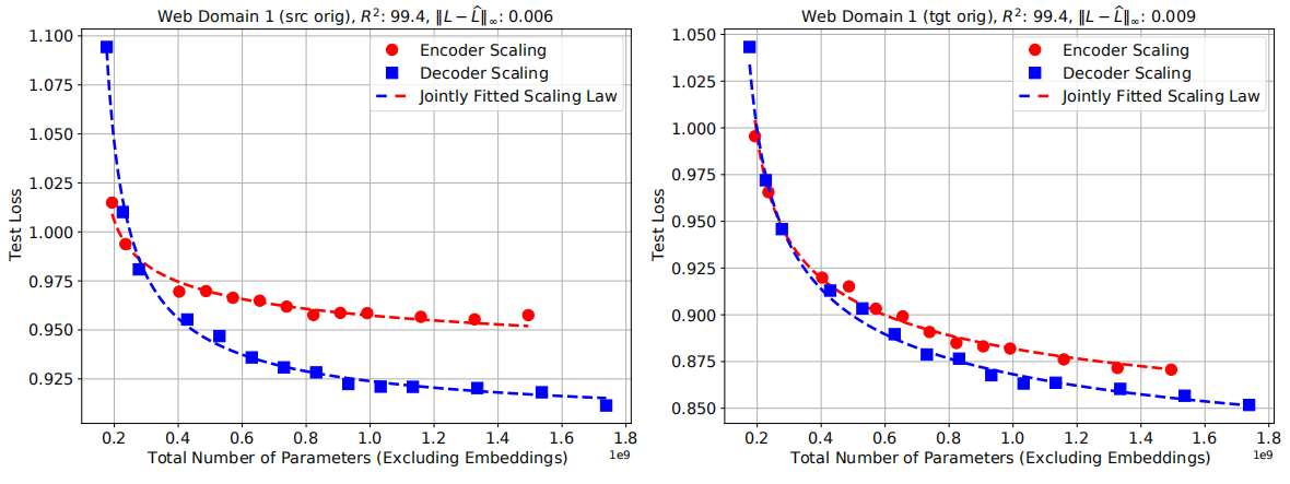
As we can see, the dashed line of each case fits the points perfectly (variance $R^{2} = 99.4$). These dashed lines were creating using the power law of the form:

Where $N$ is the total number of parameters outside of embedding / softmax layers and $\left( \alpha,\ p,\ L_{\infty} \right)$ are the fitted parameters of the power law which change based on the data.

Now, given a Transformer model of $\overline{N}_e$ encoder layers and $\overline{N}_d$ decoder layers trained on a certain dataset, the following formula predicts the new performance on the same dataset when the encoder layers become $N_e$ and the decoder layers become $N_d$:

Where the parameters $\left( \alpha,\ p_{e},\ p_{d},\ L_{\infty} \right)$ are achieved using the following algorithm that uses scipy.optimize.least_squares() function for curve fitting while using 'soft_l1' loss option which is a popular option to have some robustness to outliers:

def func(p, x, y):
    """
    Fitting a bi-variate scaling law.
    p: A 1-D array of dim 4, corresponding to alpha, p_e, p_d, l_inf.
    x: A matrix of dimension n \times 2. First column encoder params,
    second col decoder params.
    y: A 1-D array of log-perplexity of dim n.
    """
    x_e = NE_bar / x[:,0]
    x_d = ND_bar / x[:,1]
    return p[0] * np.power(x_e, p[1]) * np.power(x_d, p[2]) + p[3] - y


def fit_model(x, y, f_scale):
    X = x.to_numpy().copy()
    y = y.to_numpy().copy()
    if np.isnan(X).any() or np.isnan(y).any():
        raise ValueError('Data contains NaNs')
    if len(y.shape) > 1 or y.shape[0] != X.shape[0]:
        raise ValueError('Error in shapes')
    p0 = np.zeros((4 ,))
    p0[0] = 0.2 # alpha
    p0[1] = 0.4 # p_e
    p0[2] = 0.6 # p_d
    p0[3] = 1.0 # l_inf
    fit = least_squares(func, p0, loss='soft_l1', f_scale=f_scale,
        args=(X, y), max_nfev=10000, bounds=(0, 10))
return fit

Note:
The parameter $\alpha$ corresponds to the maximum loss reduction compared to the baseline model, while the parameter $L_{\infty}$ corresponds to the irreducible loss of the data.

The above formula captures the scaling behavior of the Transformer NMT models over a certain dataset. The following figure shows different values of the encoder exponent and the decoder exponent over multiple test sets:

As we can see, the decoder exponents $p_{d}$ were observed to be larger than the encoder exponents $p_{e}$. As a result, when improving the test loss is concerned, it is much more effective to scale the decoder rather than the encoder. This is contrary to the usual practice where many practitioners train NMT models with deep encoders and shallow decoders.

Now to a very important question, “what is the optimal Transformer size given a certain dataset?” The paper proposed the following formula which predicts the optimal size for both the encoder and the decoder:

Where $B$ is the total number of parameters you can afford in your organization. In addition, when optimally scaling the model, the scaling law reduces to:

Important Note:
In the paper, they found out that symmetrically scaling the encoder and decoder layers, which yields $\frac{N_{d}}{N} \approx 0.55$, is barely distinguishable from the optimal scaling scheme.

Scaling Effect on Quality

They examined the effects of scaling on the output quality as measured by BLEU score. The following figure presents the co-evolution of BLEU score and cross-entropy loss throughout the training for all of our models.

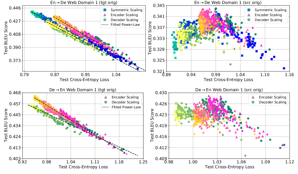
Depending on the construction of the test sets, two different empirical behaviors emerge:

• On target-original test sets, larger models are able to improve (lower) the test loss which was accompanied with consistent improvements (increases) in BLEU score. In fact, the following simple power law can capture the relation:

• On source-original test sets, larger models consistently achieve better (lower) test losses, however, beyond a certain threshold, BLEU scores begin to deteriorate.

• Also, a careful look at the left-subplots brings up another interesting trend. At similar values of the test loss, encoder-scaled models result in better generation quality compared to decoder-scaled models. This findings agrees with previous work that relied on encoder-scaling when optimizing for BLEU.