ContextNet

ContextNet is a CNN-RNN transducer model that incorporates global context information into convolution layers by adding squeeze-and-excitation modules. ContextNet was proposed by Google in 2020 and published in this paper under the same name: “ContextNet: Improving Convolutional Neural Networks for Automatic Speech Recognition with Global Context”. In this paper, they followed the RNN-Transducer framework where they used ContextNet as the encoder and a single layer LSTM as the decoder.

A major difference between the RNN-based models and a CNN-based models is the length of the context. In a bidirectional RNN model, a cell in theory has access to the information of the whole sequence; while in CNN-based models cover a small window in the time domain based on the kernel size. Since ContextNet is a fully CNN-model, it uses squeeze-and-excitation (SE) layers to enhance the global context.

Let the input sequence be $x = \left( x_{1},\ …x_{T} \right)$, the ContextNet transforms the original signal $x$ into a high level representation $h = \left( h_{1},\ …h_{T’} \right)$ such that $T’ \leq T$ just like so:

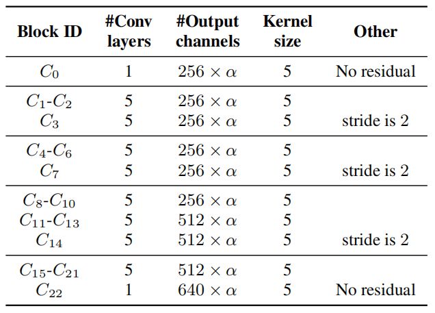
Where each $C_{i}$ refers to the $i^{\text{th}}$ convolution block and $K$ is the total number of layers. In the paper, ContextNet has 23 convolution blocks $\left( C_{0},\ …C_{22} \right)$. All convolution blocks have five layers of convolution, except $C_{0}$ and $C_{22}$, which only have one layer of convolution each as shown below in the following table:

Note:
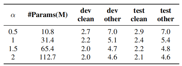
$\alpha$ is a hyper-parameter that controls the scaling of our model. Increasing $\alpha > 1$ increases the number of channels of the convolutions, giving the model more representation power with a larger model size.

Convolution Block

As shown in the following figure, a convolution block $C_{i}$ contains a number of convolutions $Conv()$, each followed by batch normalization $BN()$ and swish activation $Act()$. A squeeze-and-excitation $SE()$ block operates on the output of the last convolution layer. A skip connection with projection $Proj()$ is applied on the output of the squeeze-and-excitation block.

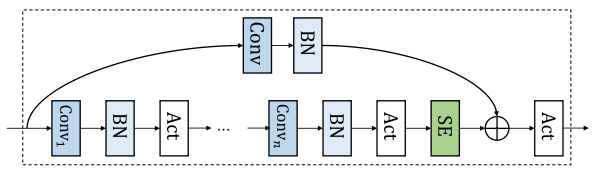
Which can be described in the following mathematical formula:

From the previous figure/formula, we can see that the convolution block in ContextNet consists of the following components:

• Convolution Function:
  ContextNet uses depthwise separable convolution, because such a design achieves better parameter efficiency without impacting accuracy. For simplicity, they used the same kernel size on all depthwise convolution layers in the network.

• Swish Activation:
  ContextNet uses swish function with $\beta = 1$ defined below; which was (according to the paper) consistently better than ReLU:

• Squeeze-and-excitation Layer:
  SE Layer or squeeze-and-excitation layer was first introduced in “Squeeze-and-Excitation Networks” paper published in 2017. It got its name because it squeezes a sequence of local feature vectors into a single global context vector, broadcasts this context back to each local feature vector, and merges the two via multiplications as illustrated below:

  
  • First, it performs global average pooling on the input $x \in \mathbb{R}^{T \times C}$ to form $\overline{x} \in \mathbb{R}^{C}$: where $T$ is the total number of time-steps in the earlier block and $C$ is the number of channels:
  \[\overline{x} = \frac{1}{T}\sum_{t = 1}^{T}x_{t}\]
  • Then, it transforms $\overline{x}$ into a global channel-wise weight $\theta\left( x \right) \in \mathbb{R}^{C}$ using two learnable weight matrices: $W_{1} \in \mathbb{R}^{C \times \frac{C}{8}}$ and $W_{2} \in \mathbb{R}^{\frac{C}{8} \times C}$, and two learnable bias vectors: $b_{1} \in \mathbb{R}^{\frac{C}{8}}$ and $b_{2} \in \mathbb{R}^{C}$.
  \[\theta\left( x \right) = \sigma\left( W_{2}\left( \text{Act}\left( W_{1}\overline{x} \right) + b_{1} \right) + b_{2} \right)\]
  • Finally, it performs an element-wise multiplication (denoted by $\circ$) of each time-frame of $x$ using this channel-wise weight $\theta\left( x \right)$:

Experiments & Results

Experiments were conducted on the Librispeech dataset which consists of 970 hours of labeled speech and an additional text only corpus for building language model. They used a $25ms$ window with a stride of $10ms$ to extract 80 dimensional filter-banks as features.

To train ContextNet, they used the Adam optimizer with learning rate with 15k warm-up steps and a peak learning rate of $0.0025$. An L2 regularization with $10^{- 6}$ weight is also added to all the trainable weights in the network. For the decoder, they used a single layer LSTM as decoder with input dimension of 640. Variational noise is introduced to the decoder as a regularization.

Also, they used SpecAugment as an augmentation method with mask parameter ($F = 27$), and ten time masks with maximum time-mask ratio ($p_{S} = 0.05$), where the maximum size of the time mask is set to $p_{S}$ times the length of the utterance. Time warping was not used.

For language model, they used a 3-layer LSTM with width 4096 trained on the LibriSpeech language model corpus with the LibriSpeech960h transcripts added, tokenized with the 1k WPM (WordPiece Model) built from LibriSpeech 960h. The LM weight $\lambda$ was tuned on the dev-set via grid search.

The following table shows summarizes the evaluation results as well as the comparisons with a few previously published systems. In the table, we can see three different configuration of ContextNet; they all have the same architecture and only differ in $\alpha$ whose value is $\left\{ 0.5,\ 1,\ 2 \right\}$ for the small, medium and large ContextNet.

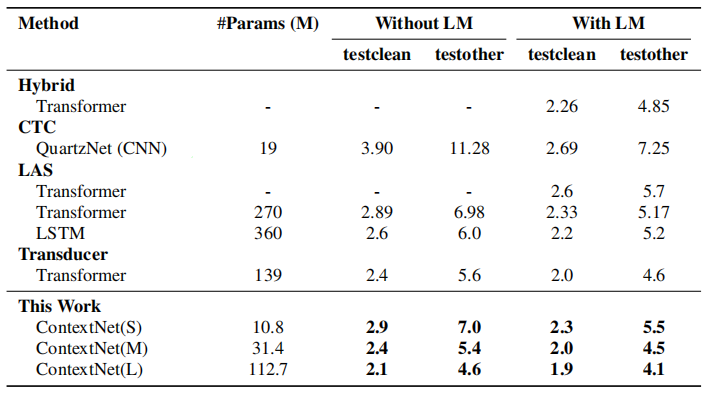
The results suggest improvements of ContextNet over previously published systems. ContextNet(L) outperforms the previous SOTA by 13% relatively on test-clean and 18% relatively on test-other. Our scaled-down model, ContextNet(S), also shows an improvement over QuartzNet, with or without a language model. Finally, ContextNet(M) only has 31M parameters and achieves similar WER compared with much larger systems.

Ablation

To validate the effectiveness of different components of the ContextNet architecture, they performed an ablation study on how these different components affects the WER on LibriSpeech; where they used ContextNet with $\alpha = 1.25$ and without SE layers as a baseline.

• SE Context: They invested different context sizes by controlling the size of the pooling window. They tried window size of 256, 512 and 1024 on all convolutional blocks. The results -shown below- shows that performance increases as the length of the context window increases.

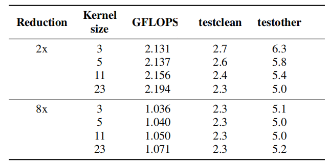
• Kernel Size and Down-sampling: They tried different kernel sizes in two different configuration (2x: half the ContextNet size, and 8x: one-eighth the ContextNet size) and the results show that down-sampling introduces significant saving in the number of FLOPS. Moreover, it actually benefits the accuracy of the model slightly.

• Model’s Width: They tried different values for which increases the width of the model. the following table demonstrates the good trade-off between model size and WER of ContextNet.