Deep Speech

Deep Speech is a well-optimized end-to-end RNN system for speech recognition created by Baidu Research in 2014 and published in their paper: Deep Speech: Scaling up end-to-end speech recognition. Deep Speech is significantly simpler than traditional speech systems, which rely on laboriously engineered processing pipelines; these traditional systems also tend to perform poorly when used in noisy environments.

Acoustic Model

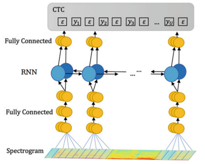
Deep Speech is an end-to-end system which means that it doesn’t need a phoneme dictionary like traditional systems. It was trained to produce transcription by predicting a sequence of character probabilities from spectrogram figures while CTC being used as an objective function:

Give a training set $X = \left\{ \left( x^{\left( 1 \right)},y^{\left( 1 \right)} \right),\left( x^{\left( 2 \right)},y^{\left( 2 \right)} \right)\text{…} \right\}$ where each utterance $x^{\left( i \right)}$ is a time-series of length $T^{\left( i \right)}$ where every time-slice $x_{t}^{\left( i \right)}$ is a vector of audio features extracted from spectrogram frames of size $t$ along with context of $C \in \left\{ 5,7,9 \right\}$ frames on each side.

The Deep Speech architecture is composed of five hidden layers:

The first three layers are fully connected layers where $W^{(l)}$ and $b^{(l)}$ are the learnable weights and bias of layer $l$ respectively.

\[{h_{t}}^{(l)} = g\left( W^{(l)}{h_{t}}^{(l - 1)} + b^{(l)} \right)\]

The fourth layer is one bi-directional RNN where $h^{(f)}$ is the forward hypothesis and $h^{(b)}$ is the backward hypothesis; both are added together to get one hypothesis:

\[h_{t}^{(f)} = g\left( W^{(4)}h_{t}^{(3)} + W_{r}^{(f)}h_{t - 1}^{(f)} + b^{(4)} \right)\] \[h_{t}^{(b)} = g\left( W^{(4)}h_{t}^{(3)} + W_{r}^{(b)}h_{t - 1}^{(b)} + b^{(4)} \right)\] \[h_{t}^{(4)} = h_{t}^{(f)} + h_{t}^{(b)}\]

The last layer is also a fully connected layer:

\[{h_{t}}^{(5)} = g\left( W^{(5)}{h_{t}}^{(4)} + b^{(5)} \right)\]

The output layer is a standard Softmax function that yields the predicted character probabilities for each time slice $t$ and character $k$ in the alphabet:

\[h_{t,k}^{(6)} = {\widehat{y}}_{t,k} = \mathbb{P}\left( c_{t} = k \middle| x \right) = \frac{\exp\left( W_{k}^{(6)}h_{t}^{(5)} + b_{k}^{(6)} \right)}{\sum_{j}^{}{\exp\left( W_{j}^{(6)}h_{t}^{(5)} + b_{j}^{(6)} \right)}}\]

All activation functions used in Deep Speech are Rectified Linear Unit (ReLU) activation functions clipped at $20$ as shown in the following formula:

\[g(z) = \min\left( \max\left( 0,\ z \right),\ 20 \right)\]

Note:
They didn’t use LSTM cells instead of RNN cells because the latter is faster as it requires less computation.

Once we have computed a prediction for $\mathbb{P}\left( c_{t} \middle| x \right)$, we compute the CTC loss $\mathcal{L}\left( \widehat{y},\ y \right)$ to measure the error in prediction. Remember that the goal of Deep Speech is to convert an input sequence $x$ into a sequence of character probabilities for the transcription $y$, with ${\widehat{y}}{t,} = \mathbb{P}\left( c{t} \middle| x \right)$, where $c_{t} \in \left{ a,b,\ \text{…}\ z,space,\ apostrophe,\ blank \right}$.

Language Model

One of the exciting components of the Deep Speech work is that the RNN model can learn a light character-level language model during the training procedure, producing “readable” transcripts even without a language model. The errors that appear tend to be phonetic misspellings of words, such as “Bostin” instead of “Boston” or “arther” instead of “are there”.

In practice, these misspellings are hard to avoid. Therefore, a character N-gram language model was integrated to the Deep Speech system. So, we need to find the sequence of characters $c = \left\{ c_{1},\ c_{2}\text{…} \right\}$ that is most probable according to both the acoustic output $\mathbb{P}\left( c \middle| x \right)$ and the character N-gram language model output $\mathbb{P}_{\text{lm}}(c)$:

\[Q(c) = log\left( \mathbb{P}\left( c \middle| x \right) \right) + \alpha\ \log\left( \mathbb{P}_{\text{lm}}(c) \right) + \beta\ word\_ count(c)\]

Where both $\alpha$ and $\beta$ are tunable parameters that control the trade-off between the acoustic model (Deep Speech) and the language model. In the paper, they maximize this objective using a highly optimized beam search algorithm, with a typical beam size $\in \left\lbrack 1000,8000 \right\rbrack$.

Note:
In the paper, they used a 5-gram language model trained on 220 million phrases of the Common Crawl, selected such that at least 95% of the characters of each phrase are in the alphabet. Only the most common 495,000 words are kept, the rest remapped to an UNKNOWN token.

Training Date

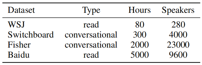
To train the Deep Speech model, they have collected an extensive dataset consisting of 5000 hours of read speech from 9600 speakers combined with some publicly data as shown in the following table:

And ensure that the “Lombard Effect” (speakers actively change the pitch or inflections of their voice to overcome noise around them) is represented in their training data (Baidu), they played loud background noise through headphones worn by a person as they record an utterance.

Also to improve the model’s performance in noisy environments, they expanded the training data by creating synthetic data. For example, if we have a speech audio track $x^{\left( i \right)}$ and a “noise” audio track $\xi^{\left( i \right)}$, then we can simulate an audio captured in a noisy environment by adding them together ${\widehat{x}}^{\left( i \right)} = x^{\left( i \right)} + \xi^{\left( i \right)}$. And to ensure a good match between synthetic data and real data, they rejected any candidate noise clips where the average power in each frequency band differed significantly from the average power observed in real noisy recordings.

Notes:

For this approach to work well, we need many hours of unique noise tracks spanning roughly to the same length as the clean speech. We can’t use less than that since it may become possible for the acoustic model to memorize the noise tracks. To overcome this, they used multiple short noise tracks and treated them as separate sources of noise before superimposing all of them: ${\widehat{x}}^{\left( i \right)} = x^{\left( i \right)} + \xi_{1}^{\left( i \right)} + \xi_{2}^{\left( i \right)} + …$

The noise environments included were the following: a background radio or TV; washing dishes in a sink; a crowded cafeteria; a restaurant; and inside a car driving in the rain.

Experiments

To train Deep Speech, they used NAG as Gradient descent optimizer with momentum factor = 0.99. For regularization, they used 5%-10% dropout rate all layers except the recurrent one. In the paper, they performed two sets of experiments.

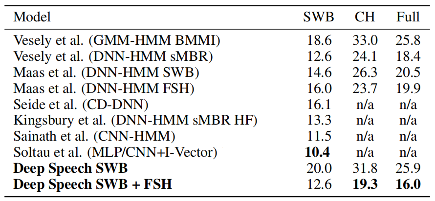
First, to compare Deep Speech with earlier models, they trained two versions of Deep Speech: Deep Speech SWB which was trained on just Switchboard dataset and Deep Speech SWB + FSH which was trained on Switchboard and Fisher datasets. And tested them on Switchboard, CallHome and Full set. The following table shows that Deep Speech achieves state-of-the-art performance.

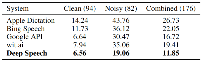
Second, To evaluate Deep Speech on noisy environment, they constructed their own evaluation set of 100 noisy and 100 noise-free utterances from 10 speakers. They trained Deep Speech on all available data; and compared it to several commercial speech systems such as: wit.ai, Google Speech API, Bing Speech, and Apple Dictation. The following table shows that Deep Speech performs way better than other commercial systems: