wav2vec

Wav2Vec is a fully convolutional neural network that that takes raw audio (wav) as input and computes a general representation (vector) that can be input to a speech recognition system. In other words, it’s a model the converts wav to vectors; hence the name. Wav2vec was created by Facebook AI Research in 2019 and published in this paper: Wav2Vec: Unsupervised Pre-Training For Speech Recognition. The official code for this paper can be found as part of Fairseq framework.

As the paper’s name suggests, unsupervised pre-training is used to the model’s performance on speech recognition. According to the paper, the speech recognition task is performed in two steps; each step will be processed by a certain model:

• Pre-training model (wav2vec):
  **A model that takes a raw audio data as input and returns some feature vectors as an output. We call these feature vectors, “contextualized representations”.

• Acoustic model:
  A model that takes these vectors as input and return a sequence of characters as output.

wav2vec: Pre-training Model

Pre-training is the fact of training the model on a task where lots of data are available, saving the weights, and later fine-tune it another task where there is limited data. Wav2vec is the model that is pre-trained to extract contextualized vectors from raw wav files. The following figure shows the proposed wav2vec model.

As shown in the previous figure, wav2vec consists of two networks:

• Encoder Network:
  A five-layer CNN model that embeds the audio signal $\mathcal{X}$ in a latent space $\mathcal{Z}$. The encoder layers have kernel sizes $\left( 10,\ 8,\ 4,\ 4,\ 4 \right)$ milliseconds and strides $\left( 5,\ 4,\ 2,\ 2,\ 2 \right)$ milliseconds. The encoder network encodes a $30ms$ frame of $16\ kHz$ audio sample $x_{i} \in \mathcal{X}$ with $10ms$ stride, and outputs a feature representation $z_{i} \in \mathcal{Z}$.

• Context Network:
  A nine-layer CNN model with kernel size of $3$ and a stride of $1$. The context network combines $v$ time-steps of the encoder’s output $\mathcal{Z} = \left\{ z_{i}\text{…}z_{i - v} \right\}$ to get a contextualized representations $c_{i} \in \mathcal{C}$. The total receptive field of the context network is about $210ms$.

Note:
The layers in both the encoder and context networks consist of a causal convolution with 512 channels, a group normalization layer and a ReLU non-linearity.

In this paper, they pre-trained wav2vec on the “noise contrastive binary classification” task where the model tries to distinguish between future true contextualized vector and some other false contextualized vectors called distractors. Formally, they trained wav2vec to distinguish a sample $z_{i + k}$ that is $k$ steps in the future from distractor samples $\widetilde{z}$ drawn uniformly from the the input sequence, by minimizing the contrastive loss for each step $k = \left\{ 1,\ …K \right\}$:

Where:

• $T$ is the sequence length.

• $k$ is the step size. In the paper, they chose $K = 12$.

• $\sigma\left( x \right)$ is the sigmoid function; defined as:

• $z_{i + k}\ $is the true sample while $\widetilde{z}$ is the false sample (distractor).

• $h_{k}\left( c_{i} \right)$ is a step-specific affine transformation of the context vector $c_{i}$.

• $\sigma\left( {z_{i + k}}^{\intercal}.h_{k}\left( c_{i} \right) \right)$ is the probability of $z_{i + k}$ being a true label.

• $\sigma\left( - {\widetilde{z}}^{\intercal}.h_{k}\left( c_{i} \right) \right)$ is the probability of $\widetilde{z}$ being a true label; note the negative sign at the beginning.

• $\lambda$ is set to be equal to the number of negative samples (distractors). In the paper, they used $\lambda = 10$.

After training wav2vec, the contextualized vectors $c_{i}$ produced by the context network are used as input to the acoustic model instead of the log-mel filterbank features.

Note:
For training on larger datasets, they used a model variant (“wav2vec large”) with increased capacity, using two additional linear transformations in the encoder and a considerably larger context network comprised of twelve layers with increasing kernel sizes $(2,3,\text{…},13)$. They also used skip (residual) connections.

Acoustic Model

In the paper, they used the Wav2Letter architecture implemented in the wav2letter++ toolkit as the acoustic models. For the TIMIT dataset, they created a character-based wav2letter++ setup which uses seven consecutive blocks of convolutions (kernel size 5 with 1,000 channels), followed by a PReLU non-linearity and a dropout rate of $0.7$. The final representation is projected to a 39-dimensional phoneme probability. The model is trained using the Auto Segmentation Criterion using SGD with 0.9 momentum and learning rate of $0.12$, and trained for 1,000 epochs with a batch size of 16 audio sequences.

For the WSJ benchmark, they created a 17 layer model with gated convolutions wav2letter++ setup which predicts probabilities for 31 graphemes, including the standard English alphabet, the apostrophe and period, a silence token (|) used as a word boundary, and two repetition characters (e.g. the word “ann” is transcribed as “an1”). This acoustic model was trained using plain SGD with learning rate $5.6$ as well as gradient clipping, and trained for 1,000 epochs with a total batch size of 64 audio sequences.

Experiments & Results

For pre-training, they used either the full 81 hours of the WSJ corpus, an 80 hour subset of clean Librispeech, the full 960 hour Librispeech training set or a combination of all of them. For phoneme recognition, they used TIMIT corpora which consists of just over three hours. For speech recognition, they used either Wall Street Journal (WSJ) which consists of 81 hours of transcribed audio data or Librispeech which contains a total of 960 hours of clean and noisy speech.

Pre-trained models were implemented in PyTorch in the Fairseq toolkit using Adam optimizer with a cosine learning rate schedule annealed over 40k update steps for both WSJ and the clean Librispeech training datasets or over 400k steps for full Librispeech. They started with a learning rate of $1 \times 10^{- 7}$, and then gradually warm it up for $500$ updates up to $5 \times 10^{- 3}$ and then decay it following the cosine curve up to $1 \times 10^{- 6}$.

When training acoustic models, they used early stopping and choose models based on validation WER after evaluating checkpoints with a 4-gram language model. The baseline acoustic model was trained on 80 log-mel filterbank coefficients for a $25ms$ sliding window with stride $10ms$.

The following table shows different models’ performance on WSJ test set (nov92) and validation set (nov93dev) in terms of both Label Error Rate (LER) and Word Error Rate (WER). † indicates results with phoneme-based models:

The past table shows that pre-training on unlabeled audio data can improve over the best character-based approach (Deep Speech 2) by 0.67 WER on nov92. On the other hand, wav2vec performs as well as the best phoneme-based model (Lattice-free MMI). And wav2vec large outperforms it by 0.37 WER.

Later in the paper, they wanted to measure the impact of pre-trained representations with less transcribed data. So, they trained acoustic models with different amounts of labeled training data and measure accuracy with pre-trained representations and without it by using log-mel filterbanks instead. The following table shows that pre-training on more data leads to better performance.

Ablations

In this section, we are going to talk about some of the design choices they made for wav2vec. All of the following results were obtained by wav2vec model pre-trained on the 80 hour subset of clean Librispeech and evaluated on TIMIT benchmark.

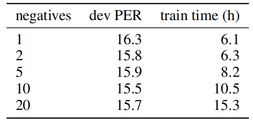
• They tested the effect of increasing the number of negative samples and they found out that it only helps up to ten samples. This happens because the training signal from the positive samples decreases as the number of negative samples increases.

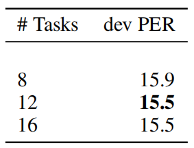
• They tested the effect of predicting more steps ahead in the future and they found out that predicting more than 12 does not result in better performance and increasing the number of steps increases training time.

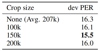
• Finally, they analyzed the effect of data augmentation through cropping audio sequences to a pre-defined maximum length. The following table shows that a crop size of 150k frames results in the best performance. Not restricting the maximum length (None) gives an average sequence length of about 207k frames and results in the worst accuracy. This is most likely because the setting provides the least amount of data augmentation.