Wav2Letter

Wav2Letter is an end-to-end model for speech recognition that combines a convolutional networks with graph decoding. Wav2letter was trained on speech signal to transcribe letters/characters, hence the name “wav-to-letter”. Wav2letter was created by Facebook in 2016 and published in this paper: Wav2Letter: an End-to-End ConvNet-based Speech Recognition System. The official code for this paper can be found in Flashlight’s official GitHub repository: wav2letter++.

Wav2Letter is a fully 1D convolutional network that has no pooling blocks. Instead, Wav2Letter leverages striding convolutions. The following figure shows the full architecture of Wav2Letter where $\text{kw}$ is the kernel width, $\text{dw}$ is the kernel stride, and the ratio is the number of input dimensions to the number of output dimensions:

Note:
Wav2Letter accepts three types of inputs: raw waveform, power spectrum and MFCC features. The previous figure is when the input is “raw waveform”. In case of either power spectrum or MFCC features, the first layer of the architecture is removed.

Given $\left( x_{t} \right)_{t = 1,2,…T_{x}}$ an input sequence with $T_{x}$ frames of $d_{x}$ dimensional vectors, a convolution with kernel width $\text{kw}$, stride $\text{dw}$ and $d_{y}$ frame size, bias of $b_{i} \in \mathbb{R}^{d_{y}}$ and weights of $w \in \mathbb{R}^{d_{y} \times d_{x} \times \text{kw}}$, it computes the following:

After that in the paper, they used an activation function of either HardTanh or ReLU which both lead to similar results:

Finally, the last layer of our convolutional network outputs one score per letter in the letter dictionary of $30$ characters: the standard English alphabet plus the apostrophe, silence, and two special “repetition” graphemes which encode the duplication (once or twice) of the previous letter. Compared to Deep Speech 2 model, wav2letter has a simpler architecture with 23 millions of parameters while Deep Speech 2 has around 100 millions of parameters.

ASG Criterion

ASG stands for “Automatic Segmentation Criterion” which is an alternative loss function to the CTC criterion. Before getting into ASG, let’s first recap how CTC works, CTC assumes that the acoustic model outputs probability scores (normalized) for each audio frame. And to detect the separation between two identical consecutive letters in a transcription, a “blank” character $\phi$ was introduced. The following graph shows all the acceptable sequences of “cat” word.

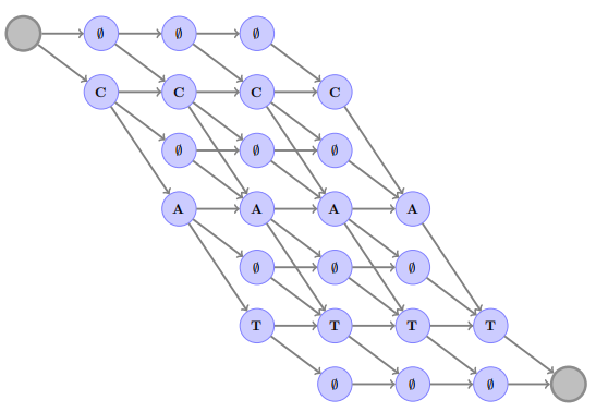
At each time step $t$, each node of the graph is assigned with the corresponding log-probability $f_{t}$ by the acoustic model. CTC aims at maximizing the “overall” graph $\mathbb{G}$ score by minimizing following score:

ASG is an alternative to CTC with three main differences:

• No blank labels:
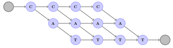
  If we removed this character, we will have a simpler vocabulary. And modeling letter repetitions can be easily replaced by repetition character like “hel2o” instead of “hello”. For example, the following graph shows all the acceptable sequences of “cat” which is way simpler than the one used with CTC:

• No normalized scores on the nodes
  In the case of CTC, the output of the acoustic model is a log-likelihood probability which is normalized per frame. Normalizing the scores on the frame-level causes “label bias”.

• Global normalization instead of frame-level normalization
  So, it considers the full fully connected graph of all possible letters shown below:

Putting all these changes together means that the ASG tries to minimize the following score where $g_{\pi_{i} \rightarrow j}()$ is a transition score model to jump from letter $i$ to letter $j$:

And the decoder they build in the paper attempts to maximize the following:

Where $P_{\text{lm}}\left( \theta \right)$ is the probability of the language model (KenLM) given a transcription $\theta$, $\alpha$ and $\beta$ are two hyper-parameters which control the weight of the language model and the word insertion penalty respectively.

Experiments

They evaluated the model on the LibriSpeech benchmark (about 1000h of audio files) for training and validating our models. They used the original $16\ KHz$ sampling rate. The MFCC features were computed with 13 coefficients with a $25ms$ sliding window and $10ms$ stride. The power features were 257 components computed with the same sliding window/stride. All features are normalized $\left( \mu = 0,\ \sigma = 1 \right)$ per input sequence. All results reported below was obtained using the model fine-tuned to get the highest validation score with 4-gram KenLM model.

The following table shows the decoding speed in milliseconds of ASG and CTC on short sequences (input frames: 150, letter dictionary: 28, transcription size: 40) on the left side; and longer sequences (input frames: 700, letter dictionary: 28, transcription size: 200):

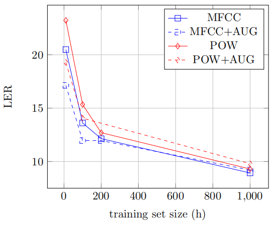
They also investigated the impact of the input feature on the performance, as well as the effect of a simple data augmentation procedure, where shifts were introduced in the input frames, as well as stretching. The following figure shows both type of features (MFCC and power) perform similarly; and the augmentation helps for small training set size. However, with enough training data, the effect of data augmentation vanishes:

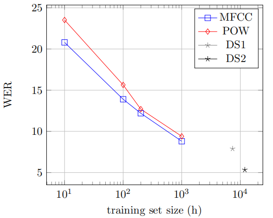
They also compared Wav2Letter with Deep Speech and Deep Speech 2 with different training sizes. The following figure reports that the WER with respect to the available training data size. As shown below, Wav2Letter performs very well against the two models despite being trained on less data:

Finally, the best scores for Wav2Letter on Librispeech for each type of features is reported in the following table: