WaveGlow

WaveGlow is a flow-based generative Vocoder capable of generating high quality speech waveforms from mel-spectrograms. WaveGlow got that name as it combines insights from Glow (flow-based generative model created by OpenAI in 2018) and WaveNet (another Vocoder model) in order to provide fast, efficient and high quality audio synthesis. WaveGlow was proposed by NVIDIA in 2018 and published in this paper under the same name: “WaveGlow: A Flow-based Generative Network for Speech Synthesis”. The official PyTorch implementation of this paper can be found on NVIDIA’s official GitHub repository: NVIDIA/waveglow. The official synthetic audio samples resulting from WaveGlow can be found in this website.

Generative Models Recap

Since WaveGlow depends heavily on Glow which is a special type of generative models called “flow-based”. Then, a recap on generative models in general will make things clearer and connect the missing pieces if found.

A generative model is a model that is able to generate new data from a certain input, this input could be a number, a vector, a matrix, or even a multi-dimensional tensor. In our context (vocoding), a generative model can be looked at as a voice actor. Given a spectrogram which is usually $(80 \times Time)$ matrix, this voice actor can generate very realistic audio waveforms or speech.

Now, we kinda understand what is a generative model. Let’s take it one step further and try to formulate that in mathematical terms. A generative model is a statistical model that tries to learn the joint probability distribution $P(X,Y)$ on given observable variable $X$ and target variable $Y$. In our context (vocoding), $X$ is the spectrogram and $Y$ is the audio waveform. In reality, there is a relation between spectrogram and waveform... right? A generative model is the model responsible for finding out that relation using the huge amount of data that we provide for it to learn.

Of course doing that is not easy, and according to this tutorial by Ian Goodfellow, there are different types/families of generative models as shown in the following figure. In this part, we are going to focus on just three of them: GAN, VAE, and Flow-based models (Tractable Density).

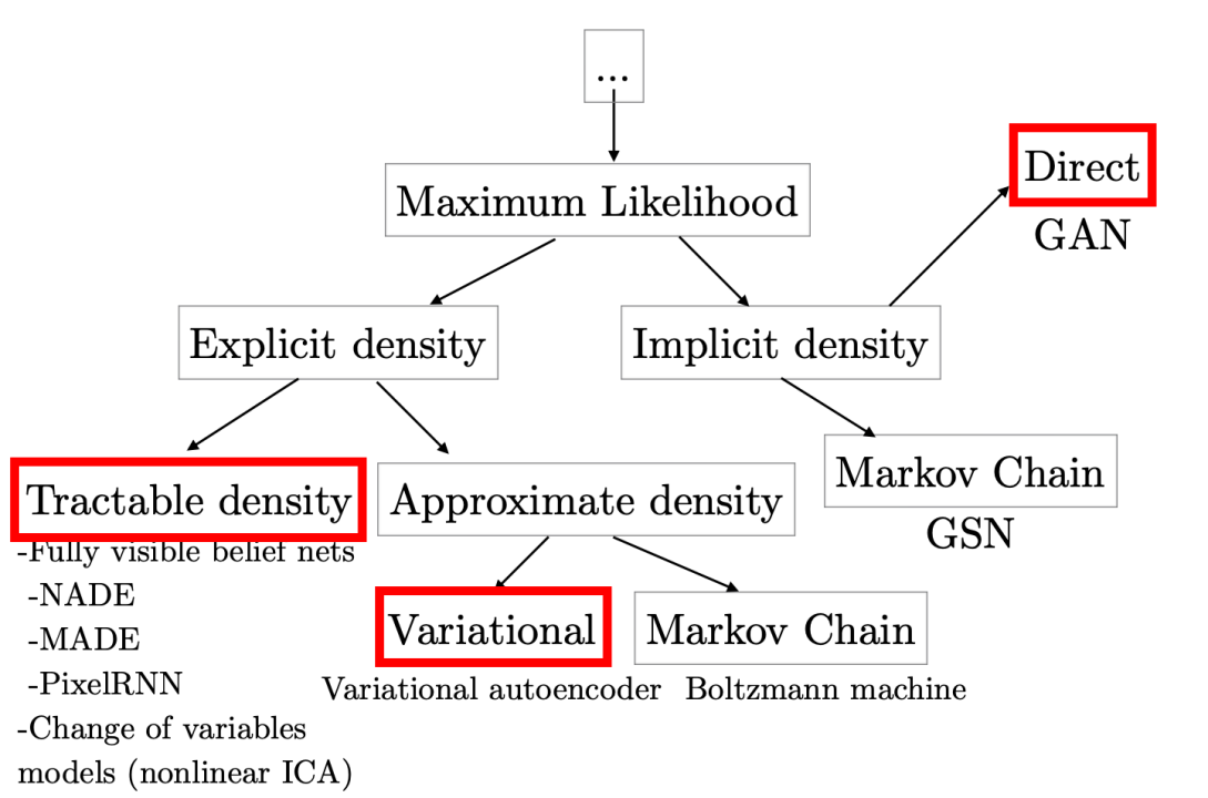
Generative models are very popular with images. So, in the next part we are going to talk about them in that context. However, as you will see this can be expanded to other contexts easily. Let’s go through them one by one:

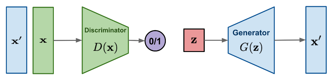
GAN:
GANs (Generative Adversarial Networks) consist of two components (generator, discriminator), only the generator is a generative model. Given 2d matrix randomly sampled from a Gaussian distribution, the generator tries to generate images using the help of the discriminator and millions of training data. In other words, the generator is trying to find a relation/map from the Gaussian distribution space to the image space.

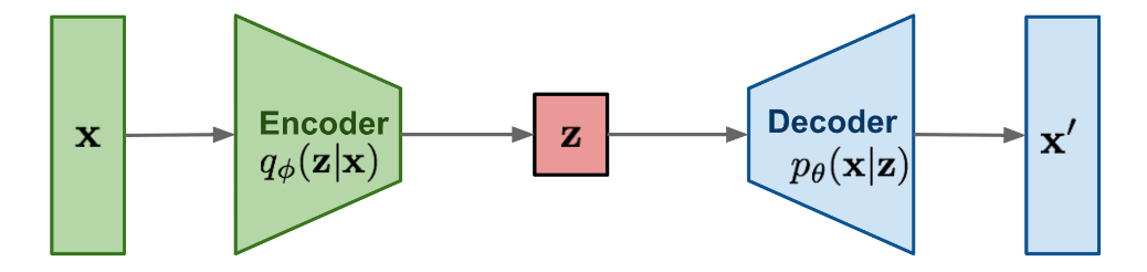
VAE:
Before talking about Variational Auto Encoders, let’s first try to understand what an Auto Encoder is. An Auto Encoder (AE) is a statistical model that is able to map image space $X$ to a lower-dimension space $Z$, and then map $Z$ back to the image space $X$. Up till this point, we don’t have any control over $Z$ which made it so noisy. To fix that issue, VAEs comes into picture and tries to make $Z$ as close as possible to a normal distribution $\mathcal{N}(0,1)$. In other words, VAEs are trying to find a relation/map from the image space to a normal distribution using the encoder part, and map the normal distribution back to the image space using the decoder part.

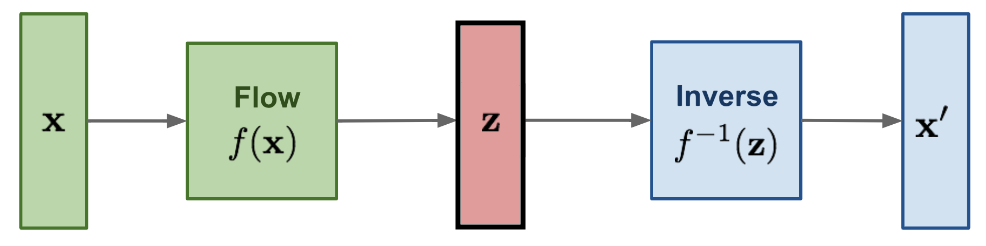
Flow-based Models:
Flow-based Models are very similar to VAEs with two main differences:
- First, the decoder (or as they call it here “inverse-flow”) is the inverse function of the encoder (or “flow”); which means that we don’t have to train two models now, we can train only one, the flow, and inverse it during inference.
- Second, the latent space $Z$ has the same dimension as the image space $X$.

Now, we have a better picture of generative models. Let’s get back to WaveGlow.

Architecture

WaveGlow is implemented using a single network, trained using only a single cost function: maximizing the likelihood of the training data, which makes the training procedure simple and stable. The whole architecture of WaveGlow can be seen in the following figure:

For the forward pass, this model takes groups of 8 audio samples as vectors, and then perform a “squeeze” operation. So, given an input tensor of size $s \times s \times c$, the squeezing operator takes blocks of size $2 \times 2 \times c$ and flatten them to size $1 \times 1 \times 4c$, which can easily be inverted by reshaping.
Then, the model processes this input through several “steps of flow”. A step of flow here consists of an invertible 1×1 convolution followed by an affine coupling layer, both are discussed in more details later.
Finally, the model is trained to directly minimize the following negative log-likelihood objective:

\[log\ p_{\theta}(x) = - \frac{z(x)^{\intercal}z(x)}{2\sigma^{2}} + \sum_{k = 0}^{\# conv}{log\ det\left( \left| W_{k} \right| \right)} + \sum_{j = 0}^{\# coupling}{\log s_{j}(x,\ melspectrogram)}\]

Where $x$ is the input audio, $z$ is the latent variable, the first term comes from the log-likelihood of a zero-mean spherical Gaussian (read the Glow paper for more details), The $\sigma^{2}$ is the assumed variance of the Gaussian distribution, and the remaining terms account for the change of variables in both “affine coupling” and “invertible convolution” respectively.

1×1 Invertible Convolution

A 1×1 convolution with equal number of input and output channels is a generalization of a permutation operation. So, they are using these 1x1 invertible convolution layers to mix information across channels before each affine coupling layer. The weights $W$ of these convolutions are initialized to be orthonormal and hence invertible.

Affine Coupling Layer

A powerful reversible transformation where the forward function, the reverse function and the log-determinant are computationally efficient, is the affine coupling layer introduced in this paper: “Density estimation using Real NVP”. The affine coupling layer, shown in the following figure, works like so:

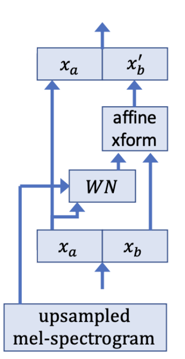
We initialize the last convolution of each NN() with zeros, such that each affine coupling layer initially performs an identity function; we found that this helps training very deep networks.
We split the upsampled mel-spectrogram into two halves along the channel dimension:

\[x_{a},\ x_{b} = split(x)\]

Then, we pass the first half $x_{a}$ to a transformation $W\ N()$. Here, $W\ N()$ does not need to be invertible. That’s why in the paper, they used WaveNet as $W\ N()$ with the only change that convolutions have 3 taps and are not causal. Then, the upsampled mel-spectrograms $x$ are added before the gated-tanh of each layer as in WaveNet.

\[\left( \log(s),\ t \right) = W\ N\left( x_{a},\ x \right)\]

Then, the other half is affine-transformed:

\[{x'}_{b} = s\bigodot x_{b} + t\]

Finally, the two resulting outputs are concatenated together:

\[f_{coupling}^{- 1}(x) = concat\left( x_{a},\ {x'}_{b} \right)\]

Experiments & Results

For all the experiments, they used the LJ speech data which consists of $13,100$ short audio clips of a single speaker reading passages from 7 non-fiction books. The data consists of roughly $24$ hours of speech data recorded on a MacBook Pro using its built-in microphone in a home environment, with a sampling rate of $22,050Hz$. For mel-spectrogram, they use mel-spectrograms with $80$ bins where FFT size is $1024$, hop size $25$, and window size $1024$.

They used WaveGlow model having $12$ coupling layers and $12$ invertible 1x1 convolutions. The coupling layer networks ($W\ N$) each have $8$ layers of dilated convolutions, with $512$ channels used as residual connections and $256$ channels in the skip connections. The WaveGlow network was trained using randomly chosen clips of $16,000$ samples for $580,000$ iterations using weight normalization [and the Adam optimizer, with a batch size of $24$ and a step size of $1 \times 10^{- 4}$. When training appeared to plateau, the learning rate was further reduced to $5 \times 10^{- 5}$.

For Mean Opinion Scores (MOS), they used Amazon Mechanical Turk where raters first had to pass a hearing test to be eligible. Then they listened to an utterance, after which they rated pleasantness on a five-point scale. They used $40$ volume normalized utterances disjoint from the training set for evaluation, and randomly chose the utterances for each subject. After completing the rating, each rater was excluded from further tests to avoid anchoring effects.

The following table shows the MOS results of WaveGlow in comparison to Griffin-Lim algorithm, WaveNet, and Ground Truth. From the table, you can see that none of the methods reach the score of ground truth. However, WaveGlow has the highest score.