Dual-decoder Transformer

Dual-decoder Transformer is a Transformer architecture that consists of two decoders; one responsible for Automatic Speech Recognition (ASR) while the other is responsible for Speech Translation (ST). This model was proposed by FAIR and Grenoble Alpes University in 2020 and published in this paper: Dual-decoder Transformer for Joint Automatic Speech Recognition and Multilingual Speech Translation. The official code of this paper can be found in the following GitHub repository: speech-translation.

The intuition behind it is that having different decoders specialized in different tasks may produce better results. In addition, these two tasks are complementary and can allow the decoders to help each other via a novel dual-attention mechanism where decoders attend to each other beside attending to the encoder.

Dual-decoder

Given an input sequence of speech features $x = \left( x_{1},\ x_{2},\ …x_{T_{x}} \right)$ in a specific source language, the dual-decoder model outputs a transcription $y = \left( y_{1},\ y_{2},\ …y_{T_{y}} \right)$ in the same language as the input and a translation $z = \left( z_{1},\ z_{2},\ …z_{T_{z}} \right)$ in $M$ different target languages. In the following equations, we are considering $M = 1$ for simplicity:

The dual-decoder transformer jointly predicts the transcript and translation in an autoregressive (left-to-right) fashion according to the following formula:

In the previous equation, we assumed that the two decoders start at the same time. In practice, one might advance $k$ steps compared to the other which is known as the wait-k policy. For example, if ST waits for ASR to produce its first $k$ tokens, then the joint distribution becomes:

In this paper, they proposed two different architectures for the dual-decoder: Parallel Dual decoder and Cross Dual-decoder. Both are using a different attention mechanism than the one used in the original transformer paper. The new mechanism is called “dual-attention”. In the next part, we are going to discuss all these details.

Parallel Dual-decoder

In parallel dual-decoder, each decoder uses the hidden states of the other to compute its outputs, as illustrated in the following figure. The encoder used is almost the same as the encoder of the original Transformer except that the embedding layer; it is a small convolutional neural network (CNN) of two layers with ReLU activations and a stride of 2, which reduces the input length by 4.

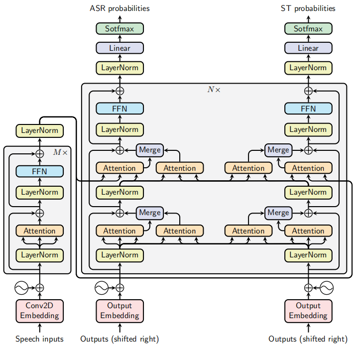
The dual-attention layer receives $Q$ from the main branch and $K,\ V$ from the other decoder at the same level/depth.

Cross Dual-decoder

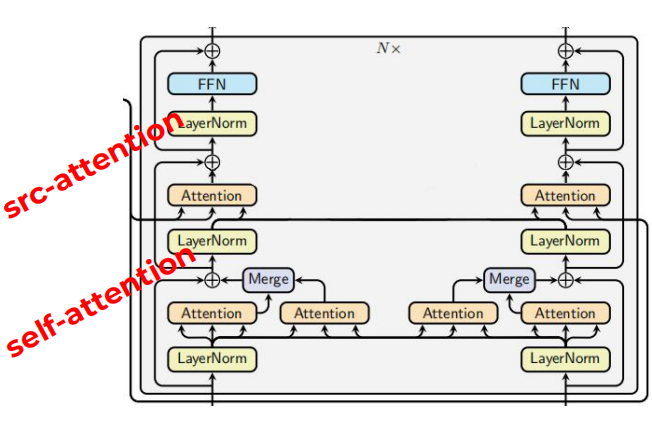
In cross dual-decoder, each decoder uses the hidden states of the other to compute its outputs, as illustrated in the following figure. The encoder used is almost the same as the encoder of the original Transformer except that the embedding layer; it is a small convolutional neural network (CNN) of two layers with ReLU activations and a stride of 2, which reduces the input length by 4.

The dual-attention layer receives $Q$ from the main branch and $K,\ V$ from the other decoder at the same lower depth.

Note:
The only difference between parallel and cross dual-decoder is how to get $K,\ V$ vectors. Parallel uses the other decoder at the same level while cross uses the other decoder at the lower level. Thanks to that, each prediction step can be performed separately on the two decoders of the cross dual-decoder which decompose the dual-decoder formula discussed earlier to:

\[h_{s}^{y} = \text{Decoder}_{\text{asr}}\left( y_{< s},\ z_{< t},\ \text{Encoder}\left( x \right) \right) \in \mathbb{R}^{d_{y}}\] \[\ h_{t}^{z} = \text{Decoder}_{\text{st}}\left( y_{< s},\ z_{< t},\ \text{Encoder}\left( x \right) \right) \in \mathbb{R}^{d_{z}}\]

Other Variants

In this section, we are going to talk about different variants of the dual-decoder Transformers used in the paper’s experiments:

• Asymmetric dual-decoder:
  Instead of using all the dual-attention layers, one may want to allow a one-way attention: either ASR attends ST or the inverse, but not both. For example, ASR attends to ST in the following parallel decoder:

• At-self / At-source dual-attention:
  In each decoder block, there are two different attention layers, which we respectively call self-attention (bottom) and source-attention (top). They tried to use either the bottom one which is called “at-self dual decoder” or the top one which is called “at-source dual decoder”. The following figure is “at-self” parallel dual decoder:

Merge Operator

The Merge operator, shown in the previous two figures, combine the outputs of the main attention $H_{\text{main}}$ and the dual-attention $H_{\text{dual}}$:

In the paper, they experimented two different merging operators:

• Weighted sum:
  Where $\lambda$ is a hyper-parameter that could be fixed or learnable.

• Concatenation:

Training & Decoding

They trained the model using the following objective; which is a weighted sum of the cross-entropy ASR and ST losses. They set $\alpha = 3$ because they favor the speech translation since it’s difficult to train because of the multilinguality.

Training data is sorted by the length of the frame where each batch contains roughly the same frame length from all languages. To differentiate between languages, a language-specific token is prepended to the target sentence.

When decoding, they use a single joint beam instead of using one separate beam for each task. In this beam search strategy, each hypothesis includes a tuple of ASR and ST sub-hypotheses. The two sub-hypotheses are expanded together and the score is computed based on the sum of log probabilities of the output token pairs.

Note:
One weakness of this beam approach is that it can happen that some transcription ${\widehat{y}}_{t}$ has a dominant score that it is selected for all the hypotheses while . In other words, we will have one transcription with different translations.

Experiments & Results

All the following experiments use the same model with a single12-layer encoder and two 6-layer decoders on MuST-C dataset. Transcriptions and translations were normalized and tokenized using the Moses tokenizer. The transcription was lower-cased and the punctuation was stripped. A joint BPE with 8000 vocabulary was learned on the concatenation of the English transcription and all target languages.

To extract features from the audio files, they used Kaldi to extract 83-dimensional features (80-channel log Mel filter-bank coefficients and 3-dimensional pitch features) which were normalized by the mean and standard deviation computed on the training set. Finally, for decoding, they used a beam size of $10$ with length penalty of $0.5$.

The following table shows the BLEU and WER scores of three main groups on the MuST-C dev set. These three groups are Independent where decoders don’t share information knowing that Independent++ uses 8-layer decoders instead of 6. crx is the Cross dual-decoder and par is the Parallel dual-decoder. Also, the superscript R3 means that ASR is 3 steps ahead of ST, while T3 means that ST is 3 steps ahead of ASR.

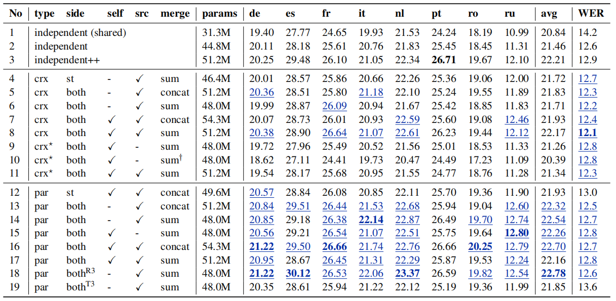
Under the same configurations in the previous table, we can see that:

• (line 5 vs. line 13) & (line 6 vs. line 14) & (line 7 vs. line 16):
  Parallel models outperform their cross counterparts in terms of translation. However, cross models outperform their parallel counterparts in terms of speech recognition.

• (line 4 vs. line 6):
  Symmetric cross models are the same as asymmetric cross models on translation but better on ASR.

• (line 12 vs. line 16):
  Symmetric parallel models are better than asymmetric parallel models on both tasks.

• (line 14 vs. line 15):
  At-source parallel models produces better results than the at-self counterparts.

• (line 13 vs. line 14) & (line 16 vs. line 17):
  The impact of merging operators is not consistent across different models. If we focus on the parallel dual-decoder, sum is better for models with only at-source attention. And concat is better for models using both at-self and at-source attention (line 16 vs. line 17).

• (line 18 vs. line 19):
  Using wait-k policy on the ST is better (letting ASR ahead) is better than the opposite on parallel models with sum operator.

  The following table shows a comparison between this dual-decoder model and other existing models on MuST-C COMMON test set and we can see that par++ achieves state-of-the-art results. The scores were calculated by averaging five checkpoints with the best validation accuracies on the dev sets.

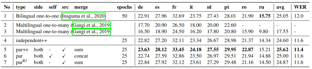
The three variants used in the previous table are:

• par++: is a parallel at-source dual-attention with sum merging operator where the decoder is 8 layers.

• par: is both at-self and at-source dual-attentions with concat merging operator.

• par^R3^: is a wait-k parallel model in which ASR is 3 steps ahead of ST