AV-HuBERT for AVSR

Audio-based automatic speech recognition (ASR) degrades significantly in noisy environments. One way to help with that, is to complement the audio stream with visual information that is invariant to noise which helps the model performance. Mixing visual stream with audio stream is known as Audio-visual speech recognition (AVSR).

Here, we are going to discuss this paper titled “Robust Self-Supervised Audio-Visual Speech Recognition” which was proposed by Meta in 2022 where authors try to fine-tune AV-HuBERT to the audio-visual speech recognition task. The official implementation of this paper can be found in Facebook Research’s official GitHub repository: facebookresearch/av_hubert. Before getting into the different details mentioned in this paper, it’s a good idea to have an overview of how AV-HuBERT works first.

AV-HuBERT Recap

AV-HuBERT stands for “Audio-Visual Hidden Unit BERT” which is a multi-modal self-supervised speech representation learning model which encodes audio and image sequences into audio-visual features. HuBERT can be considered a BERT for the “Audio” modal, and AV-HuBERT can be considered a BERT for “Audio-Visual” multi-modal systems. AV-HuBERT was proposed by Meta in 2022 and published in this paper: “Learning Audio-Visual Speech Representation by Masked Multimodal Cluster Prediction”.

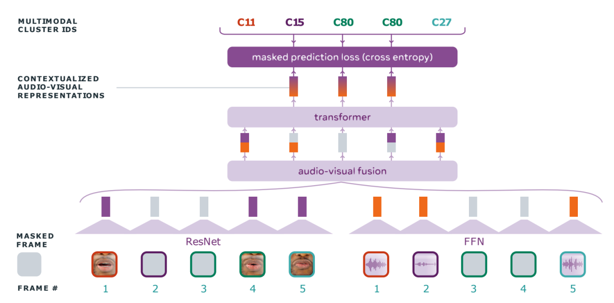
AV-HuBERT, as shown in the previous figure, is a model that combines audio features with the visual features. More formally, given an audio stream $A = \left\lbrack a_{1},\ …a_{T} \right\rbrack$ and a visual stream $I = \left\lbrack i_{1},\ …i_{T} \right\rbrack$ aligned together, AV-HuBERT is pre-trained using the following steps:

• First, both the input audio stream $A$ and the image stream $I$ are going to be masked independently using two different masking probabilities $m_{a}$ and $m_{v}$. That’s because inferring the masked targets given the audio stream is more straightforward than using the visual stream stream. So, setting a high masking probability for acoustic frames is essential to help the whole model capture the language characteristics. On the contrary, setting a high masking probability for the visual input hurts its ability to learn meaningful features.

  • The audio stream $A$ will be masked into $\widetilde{A}$ by a binary masking $M$. Specifically, $\forall t \in M$, $a_{t}$ is replaced with a masked embedding following the same masking method as HuBERT.

  • In parallel, the input image stream $I$ will be masked into $\widetilde{I}$ by a novel masking strategy where some segments in the visual stream will be substituted with random segments from the same video. More formally, given an input video $I = \left\lbrack i_{1},\ …i_{T} \right\rbrack$, an imposter segment $J = \left\lbrack j_{1},\ …j_{\mathcal{T}} \right\rbrack$ taken from the original video will be used to corrupt the input video to $\widetilde{I}$. This is done by masking $n$ intervals $M = \left\{ \left( s_i, t_i \right) \right\}_{1 \leq i \leq n}$ and replacing them with the imposter video $J$ using an offset integer $p_i$ sampled from the interval $\left\lbrack 0,\ \mathcal{T} - t_i + s_i \right\rbrack$, as shown in the following formula:

• Then, an audio encoder, which is a simple Fully-Forward Network (FFN) will be used to extract acoustic features $F^{(a)} = \left\lbrack f_{1}^{(a)},\ …f_{T}^{(a)} \right\rbrack$ from the masked audio stream $\widetilde{A}$, and in parallel a visual encoder, which is a modified ResNet-18, will be used to extract visual features $F^{(v)} = \left\lbrack f_{1}^{(v)},\ …f_{T}^{(v)} \right\rbrack$ from the visual stream $\widetilde{I}$.

• Then, these acoustic features $F^{(a)}$ will be concatenated with the visual features $F^{(v)}$ on the channel-dimension forming audio-visual features $F^{(av)}$ according to two random probabilities $p_{m}$ and $p_{a}$ useful for modality dropout; as shown in the following equation:

• Then, the acoustic-visual features are encoded into a sequence of contextualized features $E = \left\lbrack e_{1},\ …e_{T} \right\rbrack$ via the transformer encoder (BERT); followed by a linear projection layer which maps features into logits:

• Finally, AV-HuBERT is pre-trained to first identify the fake frames and then infer the labels belonging to the original frames according to the following loss function:

   Where $Z = \left\lbrack z_{1},\ …z_{T} \right\rbrack$ is the clustered representations using clustering algorithm (e.g. k-means) such that each $z_{t}$ belongs to one of $V$ different clusters (codebooks).

• The input features $h_{t}$ to the clustering algorithm change based on the training iteration:

  • For the first iteration, MFCC acoustic features extracted from the input audio stream $A$ are used.

  • For the other iterations, intermediate layers of the Visual HuBERT model are used.

Noise-Augmentation

Since AV-HuBERT was pre-trained on clean data, it’s a little bit harder for it to be robust to noisy speech recognition. A typical solution to overcome this issue is to pre-train and/or fine-tune AV-HuBERT on a synthetic audio data where we add noise to clean audio at a fixed or sampled signal-to-noise ratio (SNR).

Incorporating noise in the pre-training phase helps the model by closing the domain gap among pre-training, fine-tuning, and inference. However, the the cluster assignments are inferred from clean audio-visual speech because phonetic information, which is highly correlated with the clusters, should be invariant to noise.

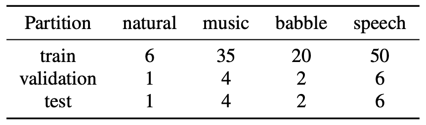
For more robustness, they used more diverse sources in their noise-augmented data, including both speech and non-speech noise in the categories of “natural”, “music” and “babble” sampled from MUSAN dataset. The total duration (in hour) of noise in each category is shown in the following table:

Noise-augmentation was done using the following steps:

• First, they select one noise category and sample a noise audio clip from its training partition.

• Then, during training they randomly mix the sampled noise at a fixed SNR of $0\ dB$ with a probability of $0.25$. At test time, they evaluate the model separately for each noise type. The testing noise clips are added at five SNR levels: $\left\{ - 10,\ - 5,\ 0,\ 5,\ 10 \right\}\ dB$.

Experiments & Results

In the paper, they used AV-HuBERT LARGE as the default model architecture for all experiments, which has $24$ transformer blocks, where each block has $16$ attention heads and $1024$/$4096$ embedding/feedforward dimensions. For fine-tuning on the audio-visual speech recognition task, they added a 9-layer randomly initialized Transformer decoder with similar embedding/feedforward dimensions. Regarding the data, they used two different datasets:

• For pre-training, they used VoxCeleb2 which has around $2,442$ hours of videos from over $6,000$ speakers and contains utterances from multiple languages. They used only the English portion. As no ground-truth language label is given in the VoxCeleb2, they used an off-the-shelf character-based ASR HuBERT model rained on Librispeech to filter non-English talks. The total amount of unlabeled data after filtering was $1,326$ hours.

• For fine-tuning, they used LRS3 (Lip-Reading Sentences 3) dataset which has around $433$ hours of audio-visual speech from over $5000$ speakers. In the original dataset, the training data is split into two partitions: “pretrain” ($403\ $hours) and “trainval” ($30$ hours). As no official development set is provided, they randomly selected $1,200$ sequences (about 1 hour) from “trainval” as the validation set which was used for early stopping and hyper-parameter tuning. They created two settings for fine-tuning the model

  • Low-resource Setting: using $30h$ of labeled videos

  • Mid-resource Setting: using $433h$ of labels.

The following table compares the WER performance of the proposed noise-augmented AV-HuBERT approach under different settings versus existing supervised AVSR models.

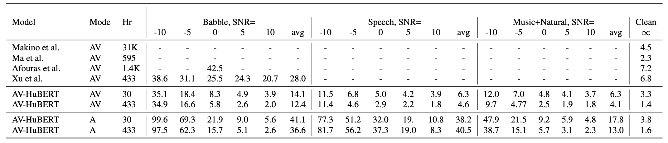
As shown in the “Babble” column, with only $30$ hours of labeled data, AV-HuBERT model outperforms other models. When using all $433$ hours labeled data for fine-tuning, the relative improvement is further increased. When the noise type is extended beyond “babble” noise, the audio-visual model consistently improves over its audio-only counterpart.

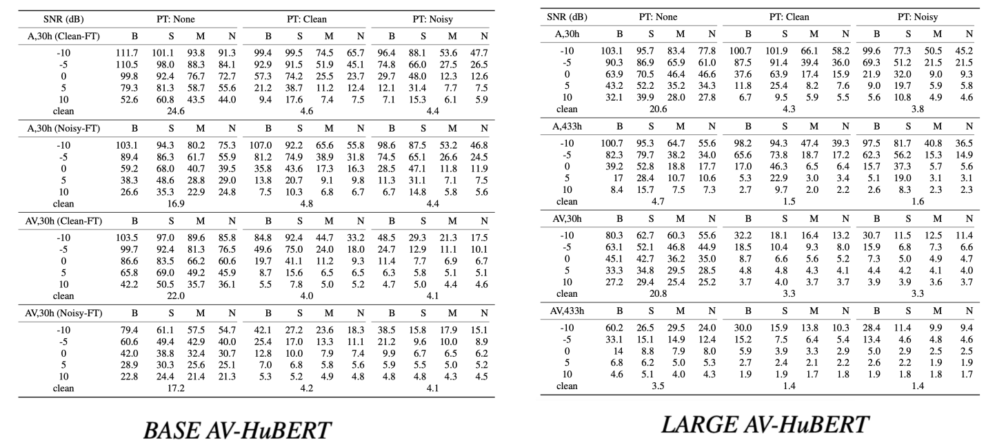
The full results of the test WER (%) score of BASE and LARGE AV-HuBERT under different levels and types of noise (B: babble, S: speech, M: music, N: natural noise):

Ablation Study

To examine the impact of pre-training (no pre-training, pretraining with clean audio, or noise-augmented pre-training) and input modality (audio or audio-visual), they performed different ablation experiments as we are going to see next:

Effect of Visual Modal & Pre-training

First, they examined the performance of AVSR models against audio-only ASR models under low-resource and mid-resource conditions by comparing audio-only vs. audio-visual HuBERT LARGE models. The following figure measure the WER (%) performance of different models under different pre-training setups:

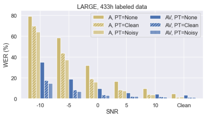
As seen in the previous figure, audio-visual models consistently outperforms audio-only models under all settings regardless of the SNR and the pre-training setup. And that shows the clear benefit of incorporating the visual stream.

Regarding the pre-training effect, AV-HuBERT pre-training brings substantial relative improvements of $78.3\%$ and $53.4\%$ on average when using 30h and 433h of labeled data, respectively. The model achieves bigger gains in the low-resource setting, which confirms the impact of the self-supervised audio-visual representations learned by the AV-HuBERT model. Regarding the noise-augmented pre-training, overall it improves the results in noisy settings compared to pre-training on clean data.

Effect of the Noise Category

Compared to “babble”, “music” and “natural” noise types, noise-augmented AV-HuBERT pre-training is more effective in overlapping “speech” noise as shown in the following figure. When comparing audio-visual and audio-only models, the visual modality provides a strong clue to “choose” the target speech track.

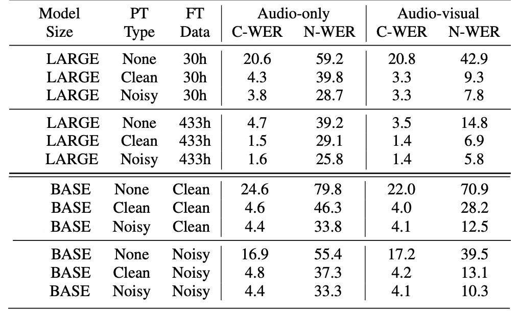
The gains from noise-augmented pre-training generalize across model architectures (BASE vs LARGE), as shown in the following table: