HuBERT

HuBERT stands for “Hidden-unit BERT”, which is a BERT-like model trained for speech-related tasks. HuBERT utilizes a novel self-supervised learning method that made its performance either matches or improves upon the state-of-the-art wav2vec 2.0 performance. HuBERT was proposed by FAIR in 2021 and published in this paper under the same name: “HuBERT: Self-Supervised Speech Representation Learning by Masked Prediction of Hidden Units”. The official code for HuBERT can be found as part of Fairseq framework on GitHub: fairseq/hubert.

In the “A nonparametric Bayesian Approach to Acoustic Model Discovery” paper, researchers have found out that the hidden units of simple clustering algorithms such as k-means exhibit non-trivial correlation with the acoustic units. So, the main idea of HuBERT is to pre-train it to be as good as k-means at clustering acoustic units before further fine-tune it on speech recognition tasks to learn both acoustic and language features from input speech.

Pre-training

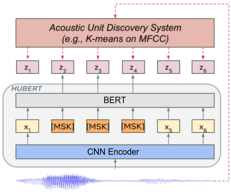
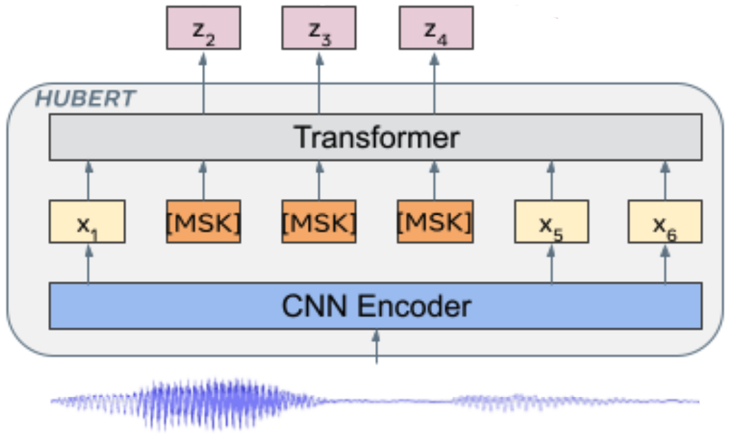
HuBERT pre-training is very similar to BERT where you mask some of the input tokens and train the model to retrieve these missing/masked tokens. One key challenge for HuBERT is that speech is continuous, unlike text which is discrete. To overcome this challenge, Acoustic Unit Discover System was used (as shown in the following figure) to cluster continuous input speech into discrete units (or codebooks) that can be masked while pre-training:

Note:
HuBERT pre-training is very similar to DiscreteBERT where both models predict discrete targets of masked regions. However, there are two crucial differences:

• Instead of taking quantized units as input, HuBERT takes raw waveforms as input to pas as much information as possible to the Transformer layers.

• Instead of using quantized units from vq-wav2vec during pre-training, HuBERT uses simple k-means targets which achieves better performance.

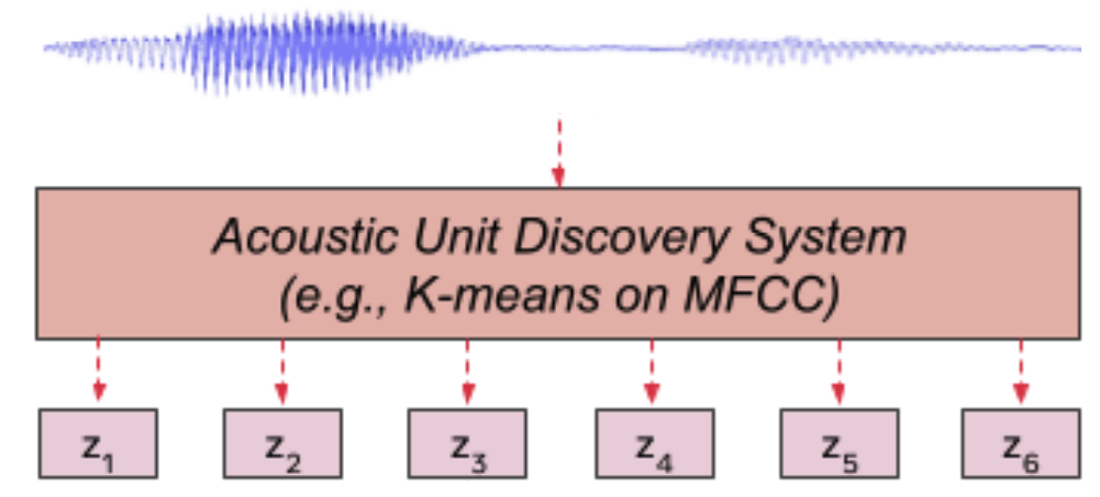
Acoustic Unit Discovery System

Let $X = \left\lbrack x_{1},\ …x_{T} \right\rbrack$ denote a speech utterance of $T$ frames, the acoustic unit discovery system uses a clustering algorithm (e.g k-means) on this input features $X$ to cluster them into a predefined number of clusters $C$. The discovered hidden units are denoted with $Z = \left\lbrack z_{1},\ …z_{T} \right\rbrack$ where $z_{t} \in \lbrack C\rbrack$ as shown in the following figure:

In the paper, they used the MiniBatchKMeans algorithm implemented in the scikit-learn package for clustering. And to improve the clustering quality, they tried two different methods:

• Cluster Ensembles:
  An ensemble of clusters can provide complementary information to facilitate representation learning. For example, an ensemble of k-means models with different codebook sizes can create targets of different classes (vowel/consonant).

• Iterative Refinement of Cluster Assignments:
  A new generation of clusters can be created using the pre-trained model from the earlier generation.

A comparison between these two techniques will be shown later.

HuBERT Model

HuBERT follows the same architecture as wav2vec 2.0 with two different parts:

• CNN Encoder:
  The convolutional waveform encoder generates a feature sequence at a $20ms$ framerate for audio sampled at $16kHz$ (CNN encoder down-sampling factor is $320x$). The audio encoded features are then randomly masked.

• BERT:
  The encoded features from the CNN Encoder get masked and sent to this model which can be considered as an acoustic BERT. Regarding masking, they used the same strategy used for SpanBERT where $p\%$ of the timesteps are randomly selected as start indices, and spans of $l$ steps are masked. And then BERT learns to predict the latent features of the unmasked and the masked input equally.

In the paper, they considered three different configurations for HuBERT: BASE, LARGE, and X-LARGE as shown in the following table. The first two follow the architectures of wav2vec 2.0 BASE and LARGE, while the X-LARGE architecture expands the model size to about 1 billion parameters, similar to the size of the Conformer XXL model.

Note:
The waveform encoder is identical for all the three configurations.

Objective

HuBERT is pre-trained to minimize the cross-entropy loss computed over masked and unmasked timesteps as $\mathcal{L}_m$ and $\mathcal{L}_u$ respectively. The final loss is computed as a weighted sum of the two terms with a hyper-parameter $\alpha$:

Where $A$ is the projection matrix appended at the end of HuBERT during pre-training; a different projection matrix is used for different cluster model. $e_{c}$ is the embedding for code-word $c$, $sim(.,\ .)$ computes the cosine similarity between two vectors, and $\tau$ scales the logit, which is set to $0.1$.

Note:
After pre-training and during fine-tuning, the projection layer(s) is removed and replaced with a randomly initialized Softmax layer. And CTC is used as a loss function for ASR fine-tuning of the whole model weights except the convolutional audio encoder, which remains frozen. The target vocabulary includes $26$ English characters, a space token, an apostrophe, and a special CTC blank symbol.

Experiments

HuBERT-BASE model was pre-trained for two iterations on the $960$ hours of LibriSpeech audio, with a batch size of at most $87.5$ seconds. The first iteration is trained for $250k$ steps on $39$-dimensional MFCC features with k-means clustering of $100$ clusters. The second iteration is trained for $400k$ steps on $768$-dimensionalfeatures extracted from the pre-trained HuBERT resulted from the first iteration.

HuBERT-LARGE and X-LARGE were pre-trained for one iteration on $60,000$ hours of Libri-light audio for $400K$ steps. The batch sizes were reduced to $56.25$ and $22.5$ seconds due to memory constraints.

For all HuBERT configurations, mask span was set to $l = 10$, and $p = 8\%$ of the waveform were randomly masked. Adam optimizer was used with $\beta = (0.9,\ 0.98)$, and the learning rate ramps up linearly from $0$ to the peak learning rate for the first $8\%$ of the training steps, and then decays linearly back to $0$. The peak learning rates were $5e^{- 4}$ for BASE, $1.5e^{- 3}$ for LARGE, and $3e^{- 3}$ for X-LARGE.

For decoding, they used wav2letter++ beam search decoder for language model-fused decoding, which optimizes the following formula where $Y$ is the predicted text, $|Y|$ is the length of the predicted text, and $w_{1}$ and $w_{2}$ denote the language model weight and word score hyper-parameters which were searched using Ax toolkit:

ASR Results

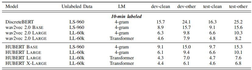
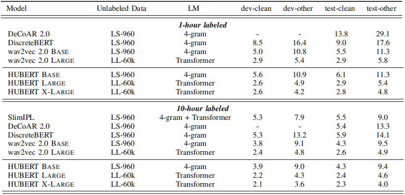
The following table shows pre-trained models which were fine-tuned on ultra-low resource setup ($10$-minutes of labeled data). It shows that HuBERT-BASE and HuBERT-LARGE can achieve lower WER than the state-of-the-art wav2vec 2.0 BASE and Large respectively.

Similar here, the superiority of HuBERT-BASE and HuBERT-LARGE over wav2vec 2.0 persists across other low-resource setups with different amounts of fine-tuning, ($1$-hour and $10$-hour) as shown in the following table:

The fine-tuning on $100$-hour of labeled data is the only exception to the rule where HuBERT-LARGE was $0.1\%$ WER higher than wav2vec 2.0 LARGE on test-clean, and HuBERT-BASE was $0.1\%$ WER higher than wav2vec 2.0 BASE as shown in the following table:

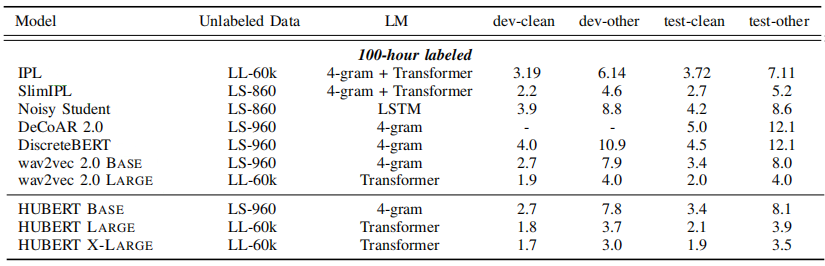
From all four previous tables, we can say that increasing the amount of labeled data and increasing the model size improve performance. HuBERT X-LARGE achieves state-of-the-art results over all test sets; demonstrating the scalability of the self-supervised pre-training method used with HuBERT.

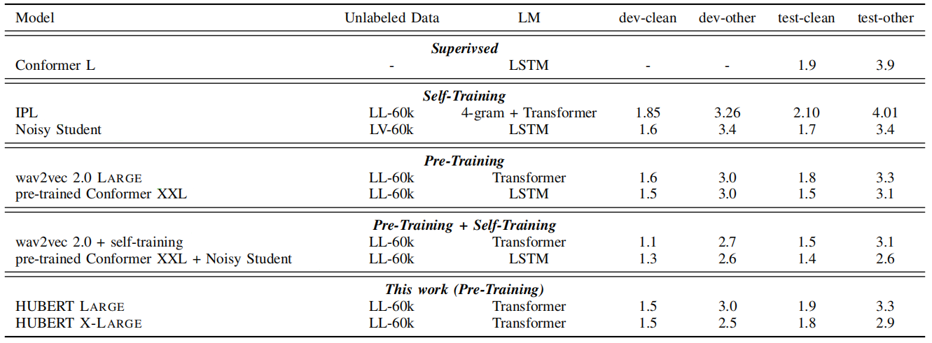
When fine-tuning HuBERT on all $960$ hours of Librispeech, it outperforms the state-of-the-art supervised and self-training methods and is on par with the pre-training results. In contrast, it lags behind with pre-training + self-training; as shown in the following table:

Clustering Analysis

In this part, we are going to discuss how they analyzed the clustering capabilities of HuBERT. Given aligned frame-level phonetic labels $\left\lbrack y_{1},\ …y_{T} \right\rbrack$ and k-means labels $\left\lbrack z_{1},\ …z_{T} \right\rbrack$, the joint distribution $p_{yz}(i,j)$ can be estimated by counting the occurrences where $y_{t} = i$ and $z_{t} = j$ divided over the total length $T$ as shown in the following formula:

And the marginal probabilities can be computed as the following:

These three formula are going to be used to calculate the following metrics:

• Clustering Stability:
  It happens when the clusters assigned don’t change by increasing the amount of data used. To measure the clustering stability, authors proposed a novel metric called “phone-normalized mutual information” that measures the clustering quality, where higher PNMI means higher quality. If the quality doesn’t change by changing the input data, this means clustering stability. PNMI can be measured using the following formula:

• Phone Purity:
  It refers to the frame-level phone accuracy, the higher the value the better the clustering is. For example, when a certain phone is aligned with multiple clusters, this means that this phone in not pure since it represents many clusters. To measure the phone purity, authors proposed the following formula:

• Cluster purity:
  It is very similar to phone purity. It refers to the frame-level cluster accuracy, the higher the value the better the clustering is. To measure the cluster purity, authors proposed the following formula:

Ablation

In the paper, authors decided to ablate some of the hyper-parameter choices to better understand its effect. First, they started by analyzing the clustering stability, then they checked the best layers for feature extractions, and finally they checked the impact of some of the hyper-parameters.

Clustering Stability

To measure the clustering stability, they considered two different setups:

• MFCC: Uses $39$-dimensional MFCC features.

• Base-it1-L6: Uses $768$-dimensional features resulted from the $6$-th transformer layer of the first iteration HuBERT-BASE model.

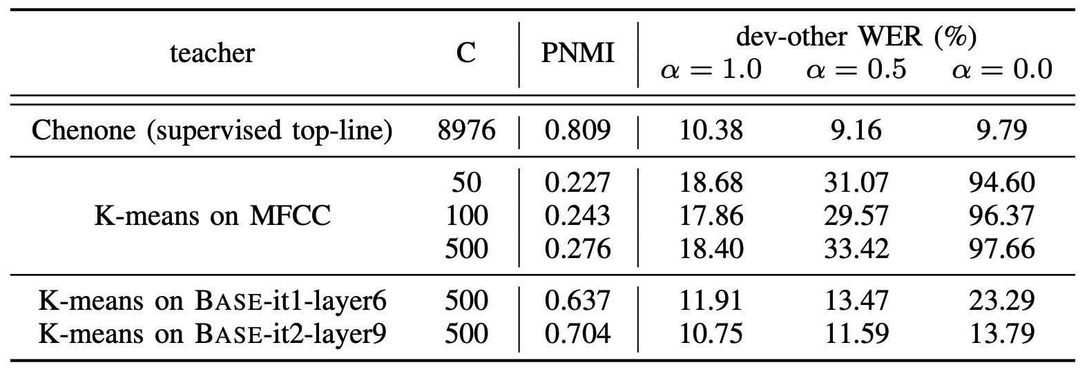
For k-means clustering, they used $100$ and $500$ clusters fitted on $1$-hour, $10$-hour, $100$-hour set from LibriSpeech. PNMI results are reported in the following table after $10$ trials:

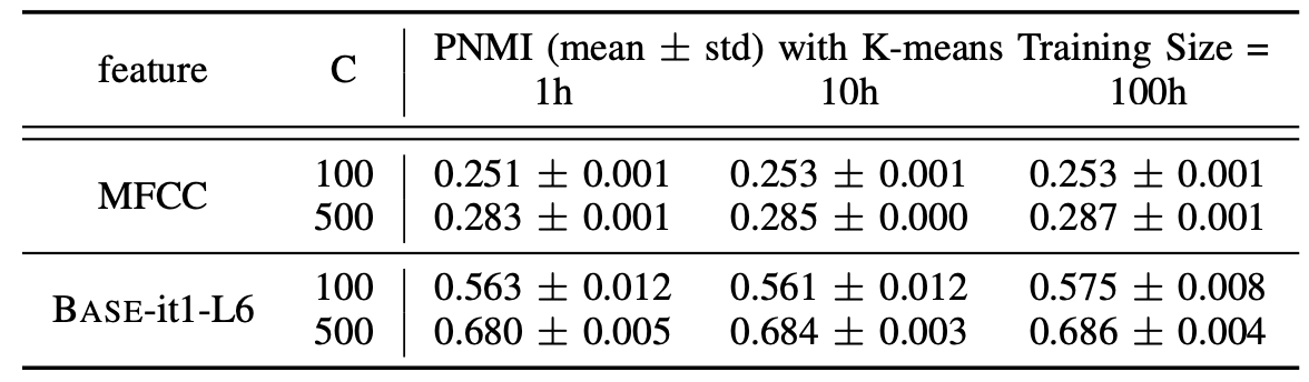
Results show that the k-means clustering is reasonably stable given the small standard deviations across different hyper-parameters and features. Also, the PNMI score is much higher when clustering on HuBERT features than clustering on MFCC features indicating that iterative refinement significantly improves the clustering quality.

Clustering Quality Across Layers

Next, they studied how each layer of the HuBERT model from each iteration performs when used for clustering to generate features for pre-training. The two $12$-layers BASE HuBERT models from the first two iterations are considered, which are referred to as BASE-it1 and BASE-it2.

BASE-it1 was pre-trained on features extracted from MFCC, while BASE-it2 was pre-trained on features BASE-it1. For each case, they used three cluster sizes ($K = \left\{ 100,500,1000 \right\}$) on a $100$-hour subset randomly sampled from the LibriSpeech training data. The clustering quality (measures in cluster purity, phone purity, and PNMI) can be shown in the following figure:

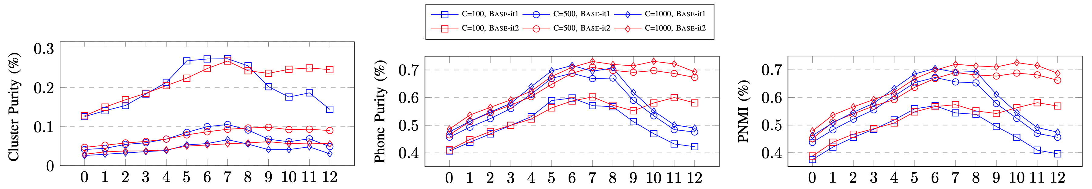
From the past results, we can conclude the following:

• BASE-it2 features are better than the BASE-it1 on phone purity and PNMI, but slightly worse on cluster purity.

• BASE-it2 model features generally improve over layers.

• BASE-it1 has the best features in the middle layers around the $6$-th layer. Interestingly, the quality of the last few layers degrades dramatically for BASE-it1, potentially because it is trained on features of worse quality, and therefore the last few layers learn to mimic their bad label behavior.

Masking-Weight Impact

To measure the impact of the masking weight hyper-parameter $\alpha$ on pre-training, they pre-trained models for $100k$ steps and fine-tuned them on the $10$-hour libri-light split using different masking weights. $\alpha = 1$ means predicting masking frames, $\alpha = 0$ means predicting unmasekd frames, and finally $\alpha = 0.5$ means predicting both masked and unmasked frames equally. WER scores on the “dev-other” set decoded with the n-gram language model using fixed decoding hyper-parameters are reported in the following table:

Results show that when learning from bad cluster assignments, computing loss only from the masked regions achieves the best performance, while the inclusion of unmasked loss results in significantly higher WERs. However, as the clustering quality improves, the model would suffer less when computing losses on the unmasked frames.

Masking Probability Impact

To measure the best value for masking probability, they tried different values where the masking probability $p = 8\%$ had the lower Word Error Rate as shown in the following figure: