T-T: Transformer Transducer

Transformer Transducer is an end-to-end speech recognition model with Transformer encoders that is able to encode both audio and label sequences independently. It is similar to the Recurrent Neural Network Transducer (RNN-T) model. The only difference is this model Transformer encoder instead of RNNs for information encoding. Transformer Transducer was proposed by Google Research in 2019 and published in this paper “Transformer Transducer: A Streamable Speech Recognition Model”. The unofficial code for this paper can be found in this GitHub repository: Transformer-Transducer.

As shown in the previous figure, The Transformer Transducer is composed of a stack of multiple identical layers. Each layer has two sub-layers:

• A multi-headed attention layer.

• A feed-forward layer.

Multi-headed Attention

The multi-headed attention layer first applies LayerNorm, then projects the input to Query, Key, and Value for all the heads. The attention mechanism is applied separately for different attention heads. The weight-averaged Values for all heads are concatenated and passed to a dense layer. Then, a residual connection is used on the normalized input and the output of the dense layer to form the final output of the multi-headed attention sublayer:

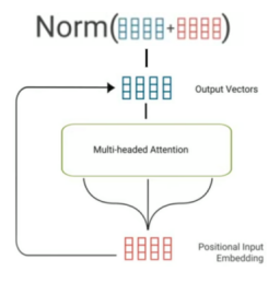
Also, a dropout on the output of the dense layer is applied to prevent overfitting.

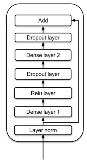
Feed-forward

As shown in the following figure, the feed-forward sub-layer applies $\text{LayerNorm}$ on the input first, then applies two dense layers. They used $\text{ReLU}$ as the activation for the first dense layer. Again, dropout to both dense layers for regularization, and a residual connection of normalized input and the output of the second dense layer:

Experiments

To evaluate this model, they used the publicly available LibriSpeech corpus which consists of 970 hours. The 10M word tokens of the text transcripts and 800M additional text only dataset were used to train a language model.

Regarding audio features, they extracted 128-channel logmel energy values from a $32ms$ window, stacked every 4 frames, and sub-sampled every 3 frames, to produce a 512-dimensional acoustic feature vector with a stride of $30ms$. SpecAugment as a feature augmentation technique was applied during model training to prevent overfitting and to improve generalization, with only frequency masking $\left( F = 50,\ mF = 2 \right)$ and time masking $\left( T = 30,\ mT = 10 \right)$.

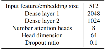
The Transformer Transducer was trained using a learning rate schedule that is ramped up linearly from $0$ to $2.5e^{- 4}$ during first 4K steps, and then held constant till 30K steps and then decays exponentially to $2.5e^{- 6}$ till 200K steps. During training, they added a Gaussian noise of $\left( µ = 0,\ \sigma = 0.01 \right)$ to model weights starting at 10K steps. Transformer Transducer was trained to output grapheme units under the same loss function as RNN-T. The full set of hyper-parameters used in the following experiments can be found in the following table:

They first compared the performance of Transformer Transducer (T-T) models with full attention on audio to an RNN-T model using a bidirectional LSTM audio encoder and with LAS as shown in the following table which shows that the T-T model significantly outperforms the RNN-T baseline despite the fact that T-T was trained much faster (≈ 1 day) than the RNN-T model (≈ 3.5 days), with a similar number of parameters:

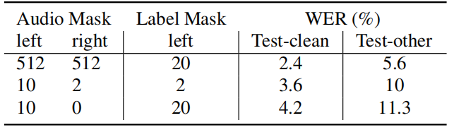
Next, they trained the model with limited attention windows over audio and text, with a view to building online streaming speech recognition systems with low latency. So, they constrained the T-T to attend to only a fixed window of the left of the current frame by masking the attention scores outside the window of the current frame. The following table shows the performance when masking N states to the left or right of the current frame. As expected, using more audio history gives better performance (lower WER):

Note:
A full attention T-T model has a window of (left = 512, right = 512).

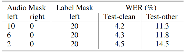
Similarly, they explored the use of limited right context to allow the model to see some future audio frames. The following table shows that with right context of 6 frames per layer, the performance is around 16% worse than full attention model:

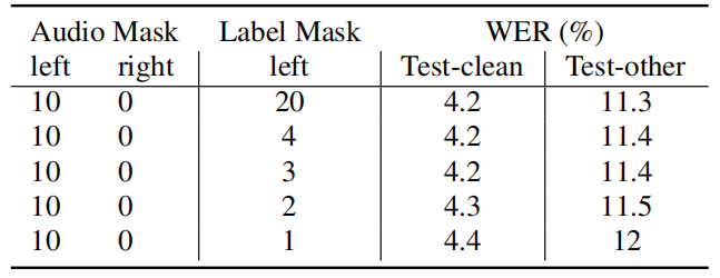
In addition, they evaluated the performance when masking the label instead of the audio features. The following table shows that constraining each layer to only use three previous label states yields the similar accuracy with the model using 20 states per layer. It shows very limited left context for label encoder is good enough for T-T model:

Finally, the following table reports the results when using a limited left context of 10 frames, which reduces the time complexity for one-step inference to a constant, with look-ahead to future frames: