wav2vec 2.0

Wav2Vec 2.0 is a self-supervised end-to-end ASR model pre-trained on raw audio data via masking spans of latent speech representations, similar to MLM used with BERT. Wav2vec was created by Facebook AI Research in 2021 and published in this paper: wav2vec 2.0: A Framework for Self-Supervised Learning of Speech Representations. The official code for this paper can be found as part of the fairseq framework on GitHub: fairseq/wav2vec2.0.

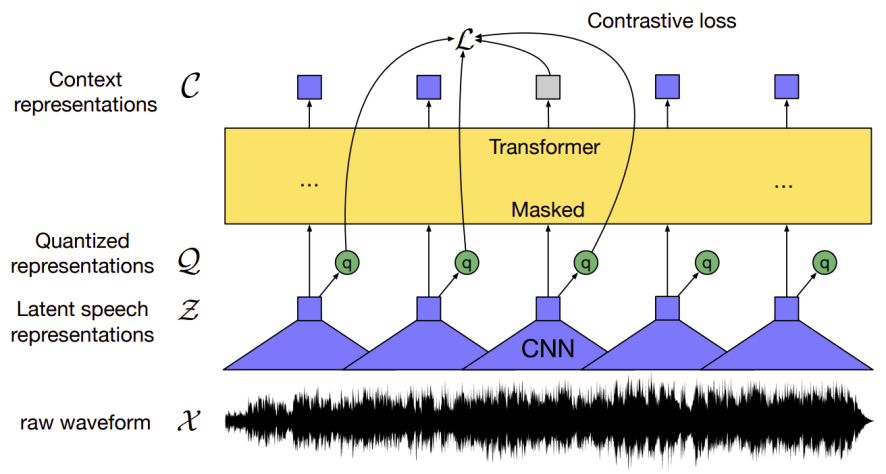
Learning purely from labeled examples does not resemble language acquisition in humans: infants learn language by listening to adults around them even before they learn to write. Wav2vec 2.0 (illustrated in the following graph) tries to mimic this idea by pre-training on unlabeled audio data first using contrastive loss, then fine-tuning on speech recognition task using labeled data with a CTC loss.

Architecture

Inspired by the wav2vec architecture and the end-to-end setup of the vq-wav2vec paper, the authors further explored a novel model architecture that consists of the following modules; which outperforms vq-wav2vec performance while using 10 times less labeled data:

Feature Encoder: Takes raw audio $\mathcal{X} = x_{1},\ x_{2},\ …\ x_{T}$ and outputs latent speech representation $\mathcal{Z} = z_{1},\ z_{2},\ …z_{T}$ for $T$ time-steps.
Transformer: Takes continuous latent representations $\mathcal{Z} = z_{1},\ z_{2},\ …z_{T}$ and outputs context representations $\mathcal{C} = c_{1},\ c_{2},\ …c_{T}$.
Quantization Module: Takes latent representations $\mathcal{Z} = z_{1},\ z_{2},\ …z_{T}$ and outputs quantized vectors $\mathcal{Q} = q_{1},\ q_{2},\ …q_{T}$.

Note:
As said before, wav2vec 2.0 is inspired by wav2vec and vq-wav2vec. However, it has the following few differences:

wav2vec 2.0 builds context representations over continuous speech representations while vq-wav2vec uses discrete speech representations.

wav2vec 2.0 uses transformers as the context network unlike . in their architecture whose self-attention captures dependencies over the entire sequence of latent representations end-to-end which is different from wav2vec.

Now, let’s talk in a little bit more details about the wav2vec 2.0 architecture.

Feature Encoder

As said earlier, the feature encoder takes normalized raw audio $\mathcal{X} = x_{1},\ x_{2},\ …\ x_{T}$ and outputs latent speech representation $\mathcal{Z} = z_{1},\ z_{2},\ …z_{T}$ for $T$ time-steps. The raw waveform input to the encoder is normalized to zero mean and unit variance.

The feature encoder consists of seven layers of temporal convolution with strides $\left( 5,2,2,2,2,2,2 \right)$ and kernel widths $\left( 10,3,3,3,3,2,2 \right)$. Each layer has $512$ channels followed by a layer normalization and a GELU activation function. The stride determines the number of time-steps $T$ returns from the encoder to the Transformer. This results in an encoder with a receptive field of of $25ms$ of audio.

Context Transformers

The output of the feature encoder is fed to a context network which follows the Transformer-encoder architecture. The original architecture of transformer encoder has a positional embedding layer. In this architecture, they used a convolution layer whose kernel size is $128$ and $16$ channels acting as positional embedding. Then, they followed the output of the convolution by a GELU and layer normalization.

In the paper, they experimented with two model configurations:

BASE:
It contains 12 transformer blocks, model dimension $768$, inner dimension (FFN) $3,072\ $and $8$ attention heads and dropout of $0.05$. We optimize with Adam, warming up the learning rate for the first $8\%$ of updates to a peak of $5 \times 10^{- 4}$ and then linearly decay it.
LARGE:
It contains $24$ transformer blocks with model dimension 1,024, inner dimension 4,096 and 16 attention heads and dropout of 0.2. We optimize with Adam, warming up the learning rate for the first $8\%$ of updates to a peak of $3 \times 10^{- 4}$ and then linearly decay it.

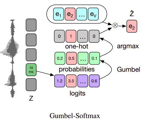
Quantization Module

For self-supervised training, they discretized the output of the feature encoder $\mathcal{Z}$ to a finite set of speech representations $\mathcal{Q}$ using Gumbel-Softmax dot quantization introduced previously in the vq-wav2vec paper.

Pre-training & Fine-tuning

To pre-train wav2vec 2.0, they randomly selected a certain proportion $p = 0.065$ of all time steps to be starting indices and then masked the subsequent $M = 10$ consecutive time steps of the feature encoder outputs $\mathcal{Z}$ before feeding them to the context network (transformer). And the objective is to identify the correct quantized latent audio representation $q_{t}$ in a set of $K$ distractors for each masked time step. The loss function for pre-training can be described in the following formula:

\[\mathcal{L} = \mathcal{L}_{m} + \alpha\mathcal{L}_{d}\]

As we can see, the loss function consists of two terms with a hyper-parameter $\alpha$ to determine the weight of each term:

Contrastive Loss $\mathcal{L}_{m}$:
Given context network output $c_{t}$ centered over masked time step $t$, the model needs to identify the true quantized latent speech representation $q_{t}$ in a set of $K + 1$ quantized candidate representations $\widetilde{q} \in \mathcal{Q}_t$ which includes $q_t$ and $K$ other distractors uniformly sampled from other masked time steps of the same utterance, $sim$ is the cosine similarity and $\mathfrak{t}$ is the temperature which is a non-negative number.

\[\mathcal{L}_{m} = - log\left( \frac{\exp\left( \frac{\text{sim}\left( c_{t},q_{t} \right)}{\mathfrak{t}} \right)}{\sum_{\widetilde{q}\sim\mathcal{Q}}^{}{\exp\left( \frac{\text{sim}\left( c_{t},q_{t} \right)}{\mathfrak{t}} \right)}} \right),\ \ \ \ \ \ sim\left( a,b \right) = \frac{a^{T}\text{.b}}{\left\| a \right\|.\left\| b \right\|}\]

Diversity Loss $\mathcal{L}_{d}$:
The diversity loss is designed to increase the use of the quantized codebook representations by encouraging the equal use of the $V$ entries in each of the $G$ codebooks:

\[\mathcal{L}_{d} = \frac{1}{\text{GV}}\sum_{g = 1}^{G}{\sum_{j = 1}^{V}{p_{g,j}.\log\left( p_{g,j} \right)}}\]

Note:
In the paper, they used $\alpha = 0.1$, $\mathfrak{t} = 0.1$, and $K = 100$.

Then, wav2vec 2.0 is fine-tuned for speech recognition by adding a randomly initialized linear projection on top of the context network into $C = 29$ classes representing the English 26 characters plus period, apostrophe and a word boundary token. Models are optimized by minimizing a CTC loss.

Labeled audio data was augmented using a modified version of SpecAugment that only masks time-steps and channels. This data augmentation delays overfitting and significantly improves the final error rates.

Experiments & Results

In the experiments, they considered two types of language models (LM): a 4-gram model and a Transformer trained on the Librispeech LM corpus. The Transformer LM contains 20 blocks, model dimension 1,280, inner dimension 6,144 and 16 attention heads. Test performance is measured with beam 1,500 for the 4-gram LM and beam 500 for the Transformer LM.

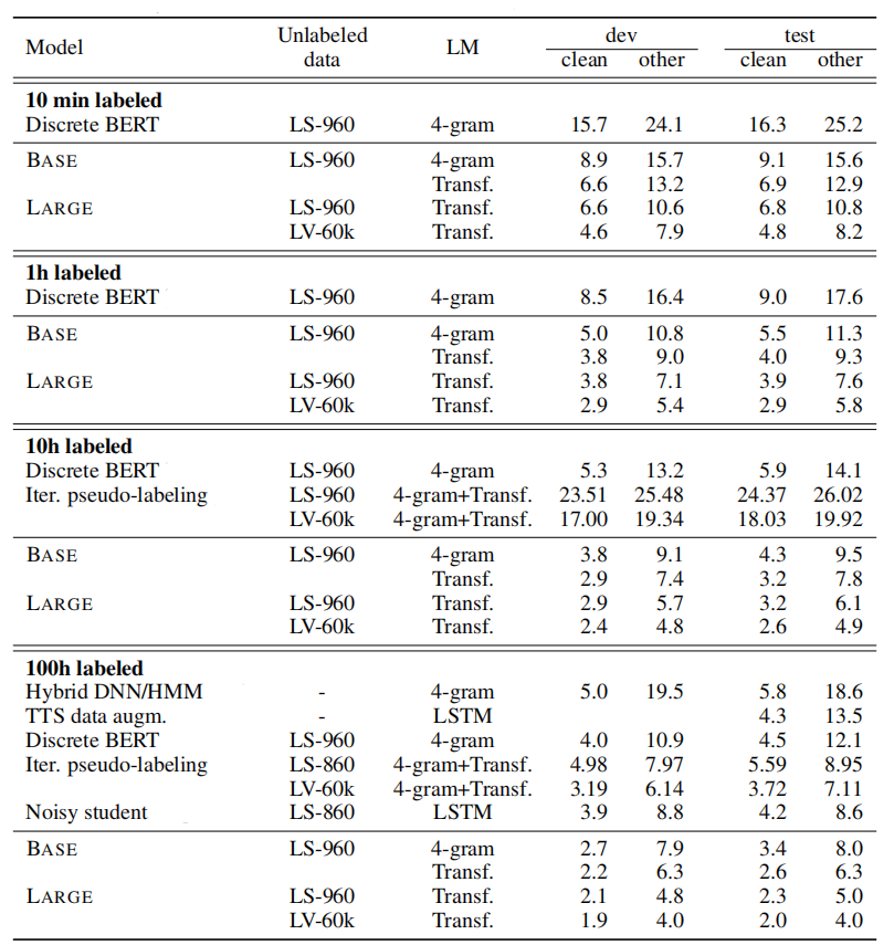
For pre-training, they used either the 960h of Librispeech corpus without transcriptions (LS-960) or the 60,000h audio data from LibriVox (LV-60k) which was 53.2k hours after preprocessing. For fine-tuning, they used two different settings of labeled data:

Low-resource setup: They used three different datasets of 10 min, 1 hour, 10 hours and 100 hours of Libri-light for this setup to have a sense of how the model is going to perform in low resource settings.
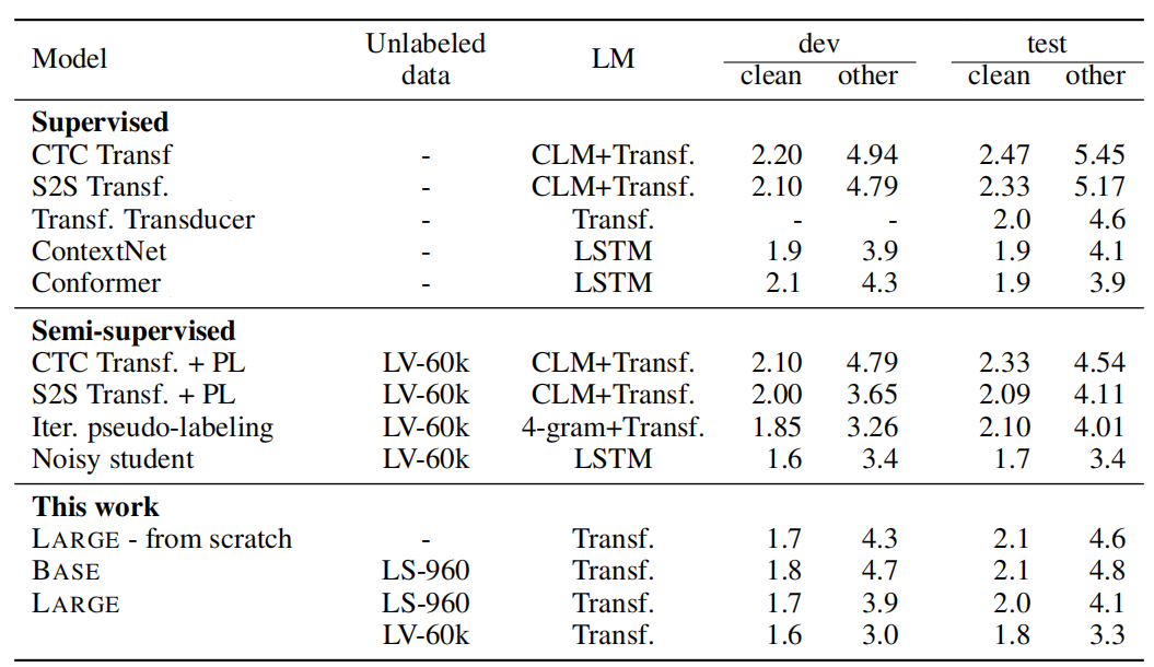
High-resource Setup: They used the 960 hours of transcribed Librispeech to assess the effectiveness of our approach in a high resource setup. The following table shows that wav2vec achieves amazing results.

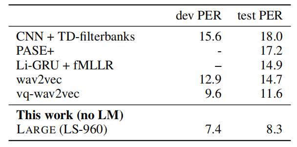
Next, they evaluated the model on TIMIT phoneme recognition by fine-tuning the pre-trained models on the labeled TIMIT training data for the 10 hour subset of Libri-light wihtout using a language model. The following table shows that this approach can achieve a new state of the art on this dataset.