SV2TTS

SV2TTS stands for “Speaker Verification to Text-to-Speech” which is a neural network-based system for text-to-speech (TTS) synthesis that is able to generate speech audio in the voice of different speakers, including those unseen during training. SV2TTS was proposed by Google in 2018 and published in this paper: “Transfer Learning from Speaker Verification to Multispeaker Text-To-Speech Synthesis”. The official audio samples outputted from this model can be found on this website. The unofficial implementation for this paper can be found in this GitHub repository: Real-Time-Voice-Cloning.

SV2TTS model can work in zero-shot learning setting, where a few seconds of untranscribed reference audio from a target speaker can be used to synthesize new speech in that speaker’s voice, without updating any model parameters. This is a big improvement over Deep Voice 2 and Deep Voice 3 which can support only speakers seen in the training data. Also, this is a big improvement over VoiceLoop which can support unseen speakers, but required tens of minutes of enrollment speech and transcripts for any new speaker.

Architecture

SV2TTS architecture can be seen in the following figure:

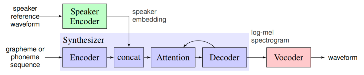
As we can see, SV2TTS consists of three independently trained components:

Speaker Encoder: A network trained on a speaker verification task using an independent dataset of noisy speech without transcripts from thousands of speakers, to generate a fixed-dimensional embedding vector from only seconds of reference speech from a target speaker.
Synthesizer: A network based on Tacotron 2 that generates a mel-spectrogram from text, conditioned on the speaker embedding.
Vocoder: An auto-regressive WaveNet-based vocoder network that converts the mel-spectrogram into time domain waveform samples.

Let’s talk about each component separately in more details:

Speaker Encoder

The foal of the speaker encoder network is to condition the synthesis network on a reference speech signal from the desired target speaker. A critical criteria for this network is to be able to capture the characteristics of different speakers using only a short recording independent of its phonetic content (text-independent) and background noise. These requirements were found in the speaker encoder model proposed earlier by this paper: “Generalized End-to-End Loss for Speaker Verification”.

As shown in the following figure, this network maps a sequence of log-mel spectrogram frames computed from a speech utterance of arbitrary length, to a fixed-dimensional embedding vector, known as d-vector (since a DNN was used to create it). This network is trained to optimize a generalized end-to-end (GE2E) speaker verification loss, so that embeddings of utterances from the same speaker have high cosine similarity, while others are far apart in the embedding space.

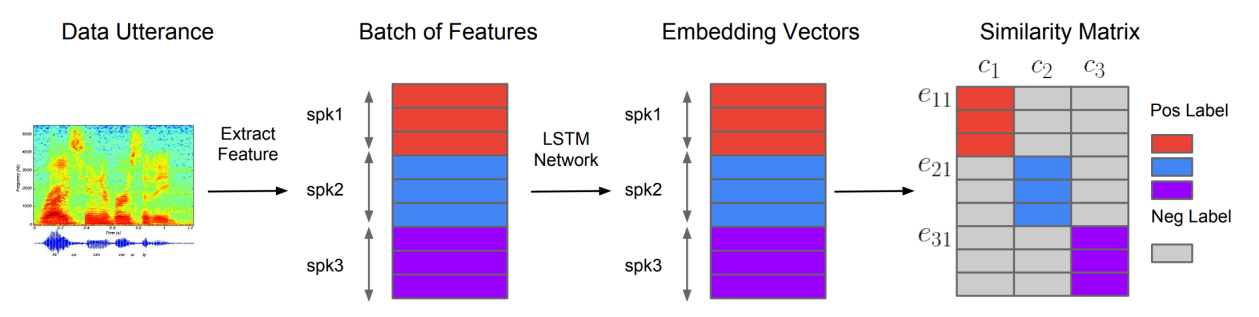
The following steps are the steps used to train this model and how to calculate the GE2E loss function:

First, the network extracts features forming a batch of utterances from $N$ different speakers where each speaker has $M$ utterances.
Then, the features extracted from each utterance $x_{\text{ij}}$ (for utterance $i$ of speaker $j$) and is fed to an (LSTM + linear layer) network denoted $f()$ with $w$ learnable parameters; resulting into vector $h_{\text{ij}}$:

\[h_{\text{ij}} = f\left( x_{\text{ij}};\ w \right)\]

The embedding vector $e_{\text{ij}}$ is defined as the L2 normalization of the previous network:

\[e_{\text{ij}} = \frac{h_{\text{ij}}}{\left\| h_{\text{ij}} \right\|_{2}}\]

The embedding for speaker $j$, is denoted as $c_{j}$ which is the centroid/average of all other utterances of the same speaker in the training data (left formula). However, in the paper, they found out that when calculating positive speakers, it’s better to remove $e_{\text{ij}}$ embedding as shown below (right formula):

\[c_{j} = \frac{1}{M}\sum_{i = 1}^{M}e_{\text{ij}},\ \ \ \ \ c_{j}^{\left( - m \right)} = \frac{1}{M - 1}\sum_{\begin{matrix} i = 1 \\ i \neq m \\ \end{matrix}}^{M}e_{\text{ij}}\]

Then, a similarity matrix between different speakers is calculated. The similarity matrix $S_{ij,\ k}$ is defined as the scaled cosine similarities between each embedding vector $e_{\text{ij}}$ to all centroids $c_{k}$; where $w$ and $b$ are learnable parameters and $w > 0$ has to be positive weight:

\[S_{ij,k} = \left\{ \begin{matrix} \text{w.}\cos\left( e_{\text{ij}},\ c_{j}^{\left( - 1 \right)} \right) + b\ \ \ \ \ \text{if }j = k \\ \text{w.}\cos\left( e_{\text{ij}},\ c_{k} \right) + b\ \ \ \ \text{otherwise} \\ \end{matrix} \right.\]

During training, we want the embedding of each utterance to be similar to the centroid of all that speaker’s embeddings, while at the same time, far from other speakers’ centroids. This was done by using the GE2E loss function defined below:

\[L_{G} = \sum_{i,j}^{}e_{\text{ij}}\]

In this paper, the network consists of a stack of $3$ LSTM layers of $768$ cells, each followed by a projection to $256$ dimensions. The final embedding is created by L2-normalizing the output of the top layer at the final frame. During training, they used audio examples segmented into $1.6$ seconds and associated speaker identity labels; no transcripts were used. Input 40-channel log-mel spectrograms are passed to the network.

During inference, an arbitrary length utterance is broken into $\mathbf{800ms}$ windows, overlapped by $\mathbf{50\%}$. The network is run independently on each window, and the outputs are averaged and normalized to create the final utterance embedding.

Note:
Although the network is not optimized directly to learn a representation which captures speaker characteristics relevant to synthesis, we find that training on a speaker discrimination task leads to an embedding which is directly suitable for conditioning the synthesis network on speaker identity.

Synthesizer

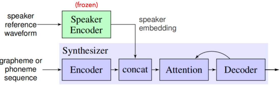
The goal of the synthesizer is to convert input features extracted from text into mel-spectrogram. In this paper, they extended the Tacotron 2 model to support multiple speakers. They did that by concatenating the target speaker embedding vector (resulting from the Speaker Encoder network) with the synthesizer encoder output at each time step as shown below:

The synthesizer is trained on pairs of text transcript and target audio. However, in this paper they map the text to a sequence of phonemes, which leads to faster convergence and improved pronunciation of rare words and proper nouns.

Target spectrogram features are computed from $50ms$ windows computed with a $12.5ms$ step, passed through an 80-channel mel-scale filter bank followed by log dynamic range compression. The loss function used was a combination between L2 loss and L1 loss. In practice, they found this combined loss to be more robust on noisy training data.

Vocoder

The goal of the vocoder is to generate audio waveforms from mel-spectrogram generated from the synthesizer. In this paper, they used WaveNet model to do so, which is composed of $30$ dilated convolution layers. The network is not directly conditioned on the output of the speaker encoder, the synthesizer network did that already.

Note to Reader:
Get back to the WaveNet post and Tacotron 2 (vocoder part) for more details.

Experiments & Results

In the paper, they used a pre-trained Speaker Encoder which was trained on an internal voice search corpus containing 36M utterances with median duration of $3.9$ seconds from 18K American speakers. During training SV2TTS, the Speaker Encoder was frozen and the the synthesizer and vocoder networks were trained separately. Experiments in the paper were performed on the following two public datasets:

VCTK: which contains $44$ hours of clean speech from $109$ speakers, the majority of which have British accents. As a pre-processing step, they down-sampled the audio to $24\ kHz$, trimmed leading and trailing silence (reducing the median duration from 3.3 seconds to 1.8 seconds), and split into three subsets: train, validation (containing the same speakers as the train set) and test (containing 11 speakers held out from the train and validation sets).
LibriSpeech: consists of the union of the two “clean” training sets, comprising 436 hours of speech from 1$,172$ speakers, sampled at $16\ kHz$. The majority of speech is US English. As a pre-processing step, they resegmented the data into shorter utterances by force aligning the audio to the transcript using an ASR model and breaking segments on silence, reducing the median duration from 14 to 5 seconds. Also, they removed the background noise.

Note:
For the VCTK dataset, whose audio is quite clean, they found that the vocoder trained on ground truth mel-spectrograms worked well. However for LibriSpeech, which is noisier, they found it necessary to train the vocoder on mel-spectrograms predicted by the synthesizer.

To evaluate the model’s performance, they constructed an evaluation set of $100$ phrases which do not appear in any training sets. To generate the speaker embedding, they randomly chose one utterance with duration of about 5 seconds. They divided the evaluation process of each datasets into two sets:

Seen: speakers that were included in the train set, 11 for VCTK and 10 for LibriSpeech
Unseen: speakers that were held out. 10 for both VCTK and LibriSpeech

For the evaluation metric, they used Mean Opinion Score (MOS) of a single rater with rating scores from 1 to 5 in 0.5 point increments, and the outputs of different models were not compared directly. The following table shows the results:

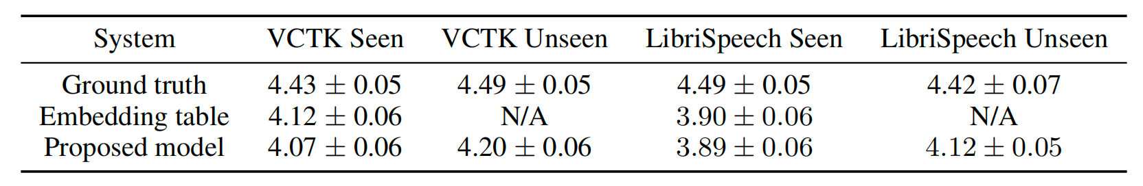
As seen from the table, SV2TTS achieved about 4.0 MOS in all datasets, with the VCTK model obtaining a MOS about 0.2 points higher than the LibriSpeech model when evaluated on seen speakers. This is the consequence of two drawbacks of the LibriSpeech dataset such as:

The lack of punctuation in transcripts, which makes it difficult for the model to learn to pause naturally.
The higher level of background noise compared to VCTK, some of which the synthesizer has learned to reproduce, despite denoising the training targets as described above.
Most importantly, the audio generated by our model for unseen speakers is deemed to be at least as natural as that generated for seen speakers. Surprisingly, the MOS on unseen speakers is higher than that of seen speakers, by as much as 0.2 points on LibriSpeech.