Tacotron 2
Tacotron 2 is a two-staged text-to-speech (TTS) model that synthesizes speech directly from characters. Given (text, audio) pairs, Tacotron 2 can be trained completely from scratch with random initialization to output spectrogram without any phoneme-level alignment. After that, a Vocoder model is used to convert the audio spectrogram to waveforms. Tacotron 2 was proposed by the same main authors that proposed Tacotron earlier in the same year (2017). Tacotron 2 was published in this paper: Natural TTS Synthesis by Conditioning WaveNet on Mel Spectrogram Predictions. The official audio samples outputted from the trained Tacotron 2 by Google is provided in this website. The unofficial PyTorch implementation for Tacotron 2 can be found in Nvidia’s official GitHub repository: NVIDIA/tacotron2.
Architecture
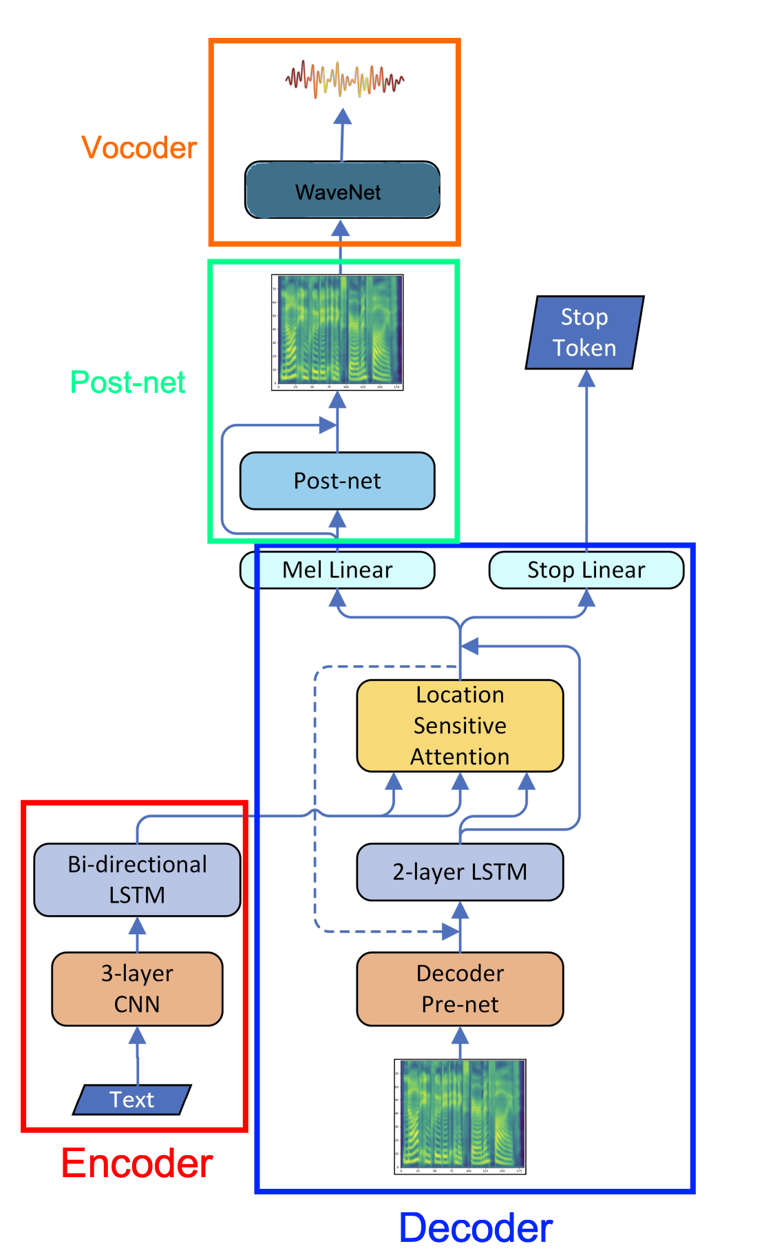
As we can see from the Tacotron 2 architecture illustrated below, Tacotron 2 consists of five main components: an Encoder, a Decoder, an AttentionMechanism, a Post-processing Network, and a Vocoder network. One clear difference between this architecture and Tacotron 1 is that they used a modified WaveNet network to convert spectrogram to Audio waveforms instead of the simple Griffin-Lim algorithm.
Note:
The convolutional layers in the whole network are regularized using dropout with probability $0.5$, and LSTM layers are regularized using zoneout with probability $0.1$.
Encoder
The goal of the encoder is to extract robust sequential representations of text. It does that by the following step:

-
Input characters are represented using a learned $512$-d character embedding.
-
These embeddings are passed through a stack of 3 convolutional layers each containing $512\ $filters with shape $5 \times 1$, i.e., where each filter spans 5 characters. After every convolutional layer, batch normalization and ReLU activations are applied. As in Tacotron, these convolutional layers model longer-term context (e.g., N-grams) in the input character sequence.
-
The output of the final convolutional layer is passed into a single bi-directional LSTM layer containing $512$ units ($256$ in each direction) to generate the encoded features.
Decoder + Attention Mechanism
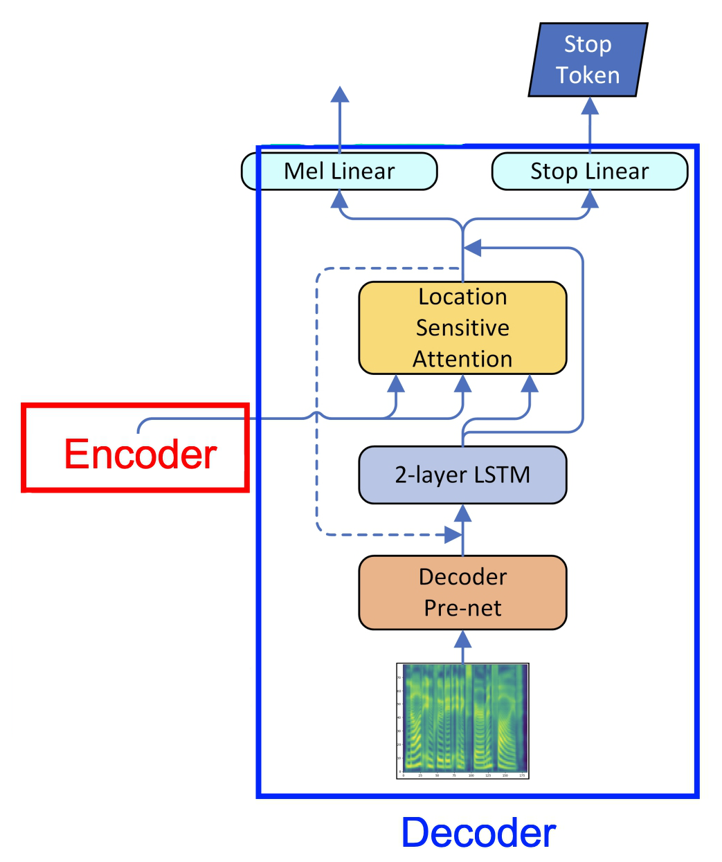
Same as Tacotron, the goal of the decoder and the attention mechanism is to align the audio frames with the textual features outputted from the encoder and result in audio spectrogram. As shown in the following figure, the decoder works like the following:
-
The first decoder step is conditioned on an all-zeros frame (the <GO> frame).
-
Similar to Tacotron, the input frame is passed to a pre-net block. The pre-net block is two fully connected layers of $256$ hidden ReLU units. In order to introduce output variation at inference time, a dropout with probability $0.5$ is applied.
-
The encoder output is consumed by an Local Sensitive Attention network which summarizes the full encoded sequence into a fixed-length context vector for each decoder output step.
-
The pre-net output and attention context vector are concatenated and passed through a stack of 2 uni-directional LSTM layers with $1024\ $units. Attention probabilities are computed after projecting inputs and location features to $128$-dimensional hidden representations. Location features are computed using $32$ 1-D convolution filters of length $31$.
-
The concatenation of the LSTM output and the attention context vector is passed into two directions in parallel:
-
The concatenation is projected through a linear transform to predict the target spectrogram frame. Unlike Tacotron, Tacotron 2 doesn’t use a “reduction factor”, i.e., each decoder step corresponds to a single spectrogram frame.
-
The concatenation is projected down to a scalar and passed through a sigmoid activation to predict the probability that the output sequence has completed. This “stop token” prediction is used during inference to allow the model to dynamically determine when to terminate generation instead of always generating for a fixed duration. It’s worth mentioning that during training there is only one “stop” signal at the end of the sequence, while other frames doesn’t have that signal.
-
-
During inference, the frame at step $t$ is fed as input to the decoder at step $t + 1$.
Post-Network
The goal of the post-network is to improve the overall reconstruction of the resulting mel-spectrogram. The post-processing network is illustrated below. It takes the decoder predicted mel-spectrogram frame as an input, then passes it through 5 convolution layers with residual connections. Each layer is comprised of $512$ filters with shape $5 \times 1$ with batch normalization, followed by $\tanh$ activations on all but the final layer.

Vocoder
Vocoder is a model that is responsible for generating audio waveforms from input features. In Tacotron 2, they used a modified version of the WaveNet architecture to invert the mel-spectrogram feature representation into time-domain waveform samples.

As in the original architecture, there are $30$ dilated convolution layers, grouped into 3 dilation cycles, i.e., the dilation rate of layer $k$ is $2k(mod\ 10)$. To work with the $12.5\ ms\ $frame hop of the spectrogram frames, only 2 up-sampling layers are used in the conditioning stack instead of 3 layers.
Instead of predicting discretized buckets with a softmax layer, they followed PixelCNN++ and Parallel WaveNet and use a 10-component mixture of logistic distributions (MoL) to generate 16-bit samples at $24\ kHz$. To compute the logistic mixture distribution, the WaveNet stack output is passed through a $\text{ReLU}$ activation followed by a linear projection to predict parameters (mean, log scale, mixture weight) for each mixture component. The loss is computed as the negative log-likelihood of the ground truth sample.
Tacotron 1 vs Tacotron 2
In the following list, I tried to summarize the subtle differences between Tacotron 1 and this model (Tacotron 2):
-
This model used LSTM cells instead of GRU cells.
-
This uses convolutional layers in the encoder and decoder instead of “CBHG” stacks.
-
This model doesn’t use reduction factor ($r$). Each decoder step corresponds to a single spectrogram frame.
-
This model uses a modified WaveNet network to convert spectrogram to Audio waveforms instead of the simple Griffin-Lim algorithm.
-
This model predicts mel-spectrogram instead of linear spectrogram.
Experiments & Results
In the paper, they trained the model on an internal US English dataset, the same dataset that Tacotron was trained on, which contains 24.6 hours of speech from a single professional female speaker. All text in our datasets is spelled out. e.g., “16” is written as “sixteen”, i.e., our models are all trained on normalized text. Unlike , training Tacotron 2 was done on two steps:
-
First, they trained the feature prediction network (whole architecture without the Vocoder part). To train this part, they used a batch size of $64$ on a single GPU with Adam optimizer with $\beta_{1} = 0.9$, $\beta_{2} = 0.999$, and $\epsilon = 10^{- 6}$ and a learning rate of $10^{- 3}$ exponentially decaying to $10^{- 5}$ starting after $50,000$ iterations. For regularization, they use L2 regularization with weight $10^{- 6}$.
-
Second, they train the Vocoder part on the ground truth-aligned predictions of the feature prediction network, where each predicted frame exactly aligns with the target waveform samples. To train this part, they used a batch size of $128$ distributed across 32 GPUs with synchronous updates, using the Adam optimizer with $\beta_{1} = 0.9$, $\beta_{2} = 0.999$, and $\epsilon = 10^{- 8}$ and a fixed learning rate of $10^{- 4}$. It helps quality to average model weights over recent updates. Therefore they maintained an exponentially-weighted moving average of the network parameters over update steps with a decay of $0.9999$. To speed up convergence, they scaled the waveform targets by a factor of $127.5$ which brings the initial outputs of the mixture of logistics layer closer to the eventual distributions.
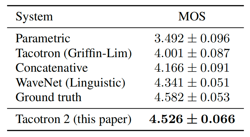
To evaluate Tacotron 2, they randomly selected 100 fixed examples from the test set of the internal dataset. Audio generated on this set are sent to a human rating service similar to Amazon’s Mechanical Turk where each sample is rated by at least 8 raters on a scale from 1 to 5 with 0.5 point increments, from which a subjective mean opinion score (MOS) is calculated. Each evaluation is conducted independently from each other, so the outputs of two different models are not directly compared when raters assign a score to them.
Similar to Tacotron, they compared Tacotron 2 with Tacotron and WaveNet alongside other models such as a parametric (based on LSTM) model from this paper: Fast, Compact, and High Quality LSTM-RNN Based Statistical Parametric Speech Synthesizers for Mobile Devices; and a concatenative system from this paper: Recent advances in Google real-time HMM-driven unit selection synthesizer. As shown in the following table, Tacotron 2 significantly outpeforms all other TTS systems and results in an MOS comparable to that of the ground truth audio:
Ablation Study
In this part, we are going to discuss the ablation experiments they performed in the paper:
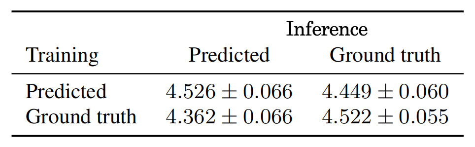
- The WaveNet component depends on the predicted features for training. In this experiment, they trained WaveNet independently on mel spectrograms extracted from ground truth audio. The following table shows that when trained on ground truth features and made to synthesize from predicted features, the result is worse than the opposite. This is due to the tendency of the predicted spectrograms to be over-smoothed and less detailed than the ground truth
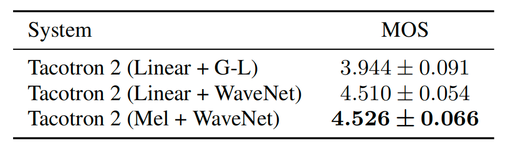
- Instead of predicting mel spectrograms, thet experimented with predicting linear spectrograms instead, like Tacotron. As shown in the following table, WaveNet produces much higher quality audio compared to Griffin-Lim. However, there is not much difference between the use of linear-scale or mel-scale spectrograms.
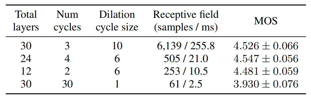
- Also, they tried different hyper-parameters for WaveNet and the following table shows that WaveNet can generate highquality audio using as few as $12$ layers with a receptive field of $10.5\ ms$, compared to $30$ layers and $256\ ms$ in the baseline model.