Improved RNN Transducer
Improved RNN-T or Improved Recurrent Neural Network Transducer is an improved version of the RNN-Transducer where a normalized jointer network is introduced to improve performance. This improved version was proposed by Bytedance AI Lab in 2020 and published in this paper: Improving RNN Transducer with Normalized Jointer Network. To further improve the performance of the RNN-T system, they used a masked Conformer model as the encoder network and the Transformer-XL as the predictor network.
They introduced this normalized jointer network is because they observed a huge gradient variance during RNN-T training such that the gradient variance is amplified for $U$ (transcription length) times on the encoder-side, and was amplified for $T$ (acoustic length) times on the predictor side. This makes the predictor and encoder hard to be optimized. To address the issue, they proposed the normalized jointer network which applies normalization for gradients at both encoder and predictor by a factor of $U$ and $T$ respectively.
Masked Conformer Encoder
Recall that the encoder of the RNN-T model works as the acoustic model where usually the input to encoder network is mel-fbank features $X = \left\{ x_{1},\ …x_{T} \right\}$, and the encoder network converts the mel-fbank features $X$ to the high-level representations $H^{\text{enc}} = \left\{ h_{1}^{\text{enc}},\ …h_{T}^{\text{enc}} \right\}$. The encoder network used in this paper is a masked Conformer model.
Recall that the Conformer major component is a stack of conformer blocks, each of which is a series of multi-headed self attention, depth-wise convolution and feed-forward layers as shown in the following figure:
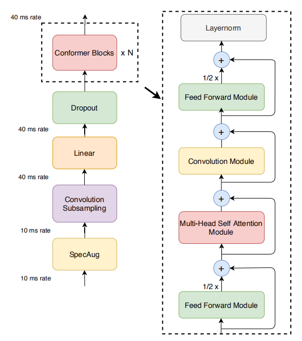
Where the multi-head self-attention module is the same multi-head self-attention attention mechanism introduced in the Transformer model which can be shown in the following equation:
\[\text{Attention}\left( Q,\ K,\ V \right) = softmax\left( \frac{QK^{\intercal}}{\sqrt{d}} \right)V\]In this paper, they modified the self-attention mechanism by adding mask $M$ to the self-attention part, and normalized by other words. The self-attention output at index $i$ can be calculated using the following equation:
\[\text{out}_{i} = \sum_{j}^{}\left( \frac{\exp\left( \frac{Q_{i}.K_{j}}{\sqrt{d}} \right).M_{\text{ij}}}{\sum_{k}^{}{\exp\left( \frac{Q_{i}.K_{k}}{\sqrt{d}} \right).M_{\text{ik}}}}.V_{j} \right)\]This mask mechanism introduced in conformer has two advantages:
-
First, adding mask to self-attention in conformer helps the convergence, especially when the training utterance is very long.
-
Second, with the mask introduced in self-attention, it is quite easy to change a non-streaming RNN-T system to a streaming fashion by masking out the right context of self attention part.
Transformer-XL Predictor
Recall that the predictor/decoder network of the RNN-T model works as the language model where usually the input to predictor network is the non-blank tokens $Y = \left\{ y_{1},\ …y_{U} \right\}$, and the predictor network converts them to the high-level representations $H^{\text{pre}} = \left\{ h_{1}^{\text{pre}},\ …h_{T}^{\text{pre}} \right\}$. The decoder network used in this paper is a Transformer-XL model.
The transformer-XL contains a segment-level recurrence mechanism, which maintains an extra-long context. Meanwhile, transformer-XL proposed a novel positional encoding scheme that adapts the sinusoid formulation in the relative positional embedding. It helps the model generalize to a longer length during evaluation.
Normalized Jointer
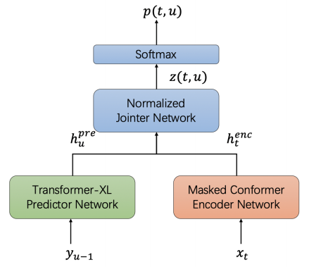
The jointer network combines the high representation from encoder $H^{\text{enc}}$ and predictor network $H^{\text{pre}}$ using a fully-connected network like so:
\[z\left( t,\ u \right) = \text{FC}\left( \tanh\left( h_{t}^{\text{enc}} + h_{u}^{\text{pre}} \right) \right)\]To understand how this equation affects the gradients during backpropagation, let’s write it with respect to each variable alone:
\[z\left( t,\ : \right) = \text{FC}\left( \tanh\left( h_{t}^{\text{enc}} + h_{:}^{\text{pre}} \right) \right)\] \[z\left( :,\ u \right) = \text{FC}\left( \tanh\left( h_{:}^{\text{enc}} + h_{u}^{\text{pre}} \right) \right)\]In the backward progress during backpropagation, gradient of $dh_t^{\text{enc}}$ and $dh_u^{\text{pre}}$ will have the following relationship with jointer network’s gradient $dz\left( t,\ u \right)$:
\[{dh}_{t}^{\text{enc}} = \sum_{u = 1}^{U}{dz\left( t,\ u \right)},\ \ \ \ \ \ \ {dh}_{u}^{\text{pre}} = \sum_{t = 1}^{T}{dz\left( t,\ u \right)}\]And usually in speech recognition task, $U$ is much bigger than $T$ which will cause unhealthy optimization of parameters. To overcome this problem, they simply divided $dh_t^{\text{enc}}$ by $U$ and divided $dh_u^{\text{pre}}$ by $T$ as shown below:
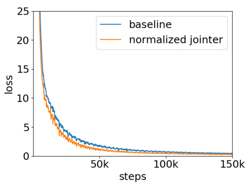
\[{dh}_{t}^{\text{enc}} = \frac{1}{U}\sum_{u = 1}^{U}{dz\left( t,\ u \right)},\ \ \ \ \ \ \ {dh}_{u}^{\text{pre}} = \frac{1}{T}\sum_{t = 1}^{T}{dz\left( t,\ u \right)}\]With this simple modification to the gradient from RNN-T’s jointer network to encoder and predictor network, the gradient norm of RNN-T’s training becomes more stable. And the validation loss decreases faster and lower as illustrated in the following figure:
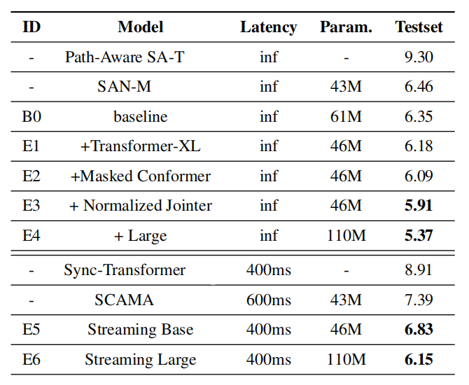
With all three proposed improvements, they achieved SOTA in the Chinese AIShell-1 dataset with $6.15\%$ and $5.37\%$ CER for streaming and non-streaming recognition respectively.