w2v-BERT

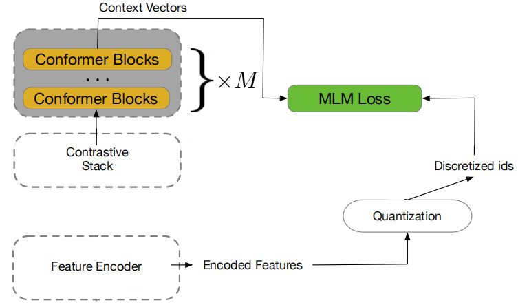
w2v-BERT combines the core methodologies of self-supervised pre-training of speech embodied in the wav2vec 2.0 model and self-supervised pre-training of language emobdied in BERT. w2v-BERT was proposed by Google Brain in 2021 and published in this paper “w2v-BERT: Combining Contrastive Learning and Masked Language Modeling for Self-Supervised Speech Pre-Training”. The w2v-BERT pre-training framework is illustrated down blow:

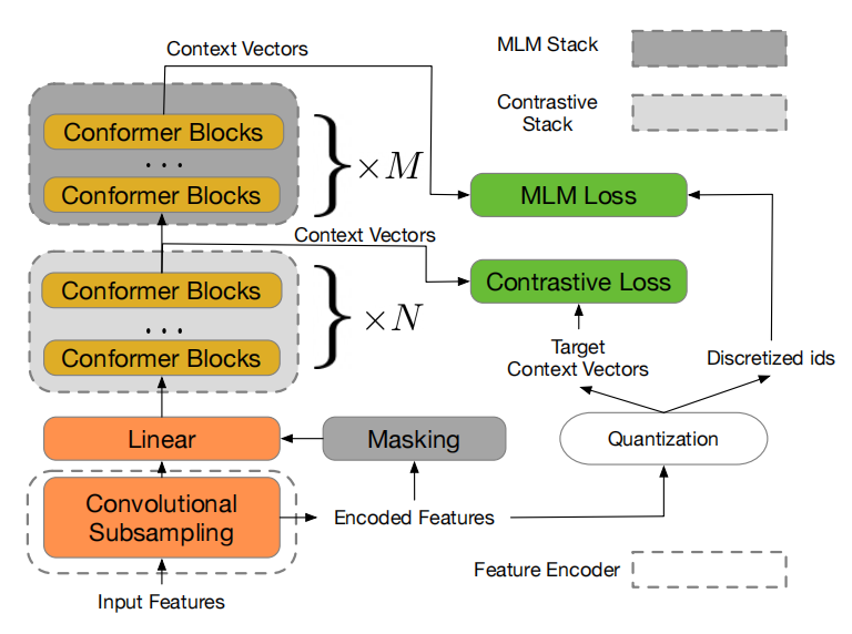
The idea of w2v-BERT is learn contextualized speech representations by using the contrastive task defined earlier in wav2vec 2.0 to obtain an inventory of a finite set of discretized speech units, and then use them as tokens in a masked prediction task similar to the masked language modeling (MLM) proposed in BERT.

From the past figure, we can see that w2v-BERT consists of three main components:

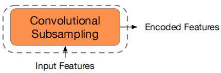
• Feature Encoder:
  The feature encoder acts as a convolutional sub-sampling block that consists of two 2D-convolution layers, both with strides $\left( 2,2 \right)$, resulting in a 4x reduction in the acoustic input’s sequence length. Given, for example, a log-mel spectrogram as input, the feature encoder extracts latent speech representations that will be taken as input by the subsequent contrastive module.

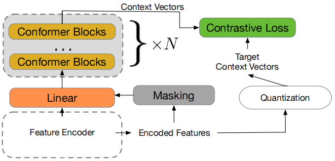
• Contrastive Module:
  The goal of the contrastive module is to discretize the feature encoder output into a finite set of representative speech units; that’s why the output of the feature encoder follows two different paths:

  • First path: It is masked, then fed into the linear projection layer followed by the stack of conformer blocks to produce context vectors.

  • Second Path: It is passed to the quantization mechanism without masking to yield quantized vectors and their assigned token IDs.

  • The quantized vectors are used in conjunction with the context vectors that correspond to the masked positions to solve the contrastive task defined in wav2vec 2.0; the assigned token IDs will be later used by the subsequent masked prediction module as prediction target.

• Masked Prediction Module:
  The masked prediction module is a stack of conformer blocks (identical to the one used with the contrastive module) which directly takes in the context vectors produced by the contrastive module and extracts high-level contextualized speech representations.

Pre-training & Fine-tuning

During pre-training only unlabeled speech data is used to train w2v-BERT to solve two self-supervised tasks at the same time weighted by two different hyper-parameters $\beta$ and $\gamma$ which were set to $1$ in the paper:

• Contrastive Loss $\mathcal{L}_{\mathbf{c}}$:
  For a context vector $c_t$ corresponding to a masked time step $t$, the model is asked to identify its true quantized vector $q_t$ from a set of $K$ distractors $\left\{ {\widetilde{q}}_1,\ {\widetilde{q}}_2,\ …{\widetilde{q}}_K \right\}$ that are also quantized vectors uniformly sampled from other masked time steps of the same utterance. This loss is denoted as $\mathcal{L}_w$, and further augment it with a codebook diversity loss $\mathcal{L}_d$ to encourage a uniform usage of codes weighted by a hyper-parameter $\alpha$. Therefore, the final contrastive loss is defined as:

• Mask Prediction Loss $\mathcal{L}_{\mathbf{m}}$:
  This is the cross entropy loss for the predicting masked context vectors. They randomly sample the starting positions to be masked with a probability of $0.065$ and mask the subsequent 10 time steps knowing that the masked spans may overlap.

During fine-tuning, a labeled data was used to train an RNN-T model where the encoder is a pre-trained w2v-BERT model, the decoder is a two-layer LSTM with a hidden dimension of $640$, and the joint network is a linear layer with Swish activation and batch normalization.

Experiments & Results

For pre-training, they use the Libri-Light unlab-60k subset, which contains about 60,000 hours of unannotated speech audio. For fine-tuning, they used the LibriSpeech 960hr subset. 80-dimensional log-mel filter bank coefficients werre used as acoustic inputs to the model. For transcript tokenization, they use da 1024-token WordPiece model that is constructed from the transcripts of the LibriSpeech training set. In the paper, they pre-trained two versions of w2v-BERT named w2v-BERT XL and w2v-BERT XXL. These two variants share the same model configuration that is summarized in the following table, and their only difference is the number of conformer blocks.

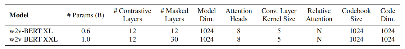
For w2v-BERT XL, they trained it with a batch size of $2048$ using the Adam optimizer with a transformer learning rate schedule. The peak learning rate is $2e^{- 3}$ and the warm-up steps are $25k$. For w2v-BERT-XXL, they trained it with the Adafactor optimizer with $\beta_{1} = 0.9$ and $\beta_{2} = 0.98$, with the learning rate schedule remaining the same. For both w2v-BERT XL and w2v-BERT-XXL, they were pre-trained for $400k$ steps, and then fine-tuned on the supervised data with a batch size of $256$.

In addition to self-supervised pre-training, in the fine-tuning stage they also employed a number of practical techniques that further improve models’ performance on ASR, like SpecAugment for data augmentation, Noisy Student Training for self-training, and language model fusion for decoding.

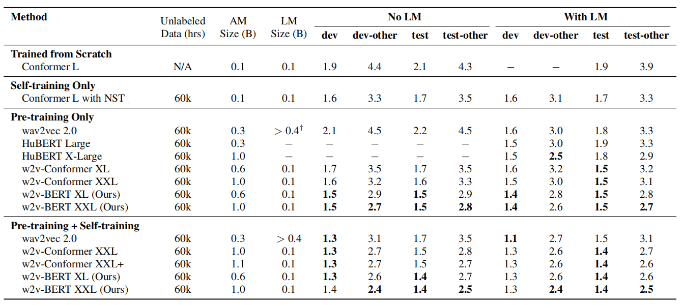
In the following table, results on the four LibriSpeech evaluation sets using the 960hr subset as the supervised data are represented. From the following table, we can see that:

• Without self-training and LM, w2v-BERT already either outperforms or matches other models with LM.

• Contrastive learning combined with masked language modeling is more effective than contrastive learning alone.