HiFi-GAN

HiFi-GAN stands for “High Fidelity General Adversarial Network” which is a neural vocoder that is able to generate high fidelity speech synthesis from mel-spectrograms efficiently more than any other auto-regressive vocoder such (e.g. WaveNet, ClariNet) or GAN-based vocoder (e.g. GAN-TTS, MelGAN). HiFi-GAN was proposed by Kakao Enterprise in 2020 and published in this paper under the same name: “HiFi-GAN: Generative Adversarial Networks for Efficient and High Fidelity Speech Synthesis”. The official implementation for this paper can be found in this GitHub repository: hifi-gan. Also, the official audio samples can be found in this website.

Architecture

HiFi-GAN consists of one generator and two discriminators: multi-period discriminator (MPD) and multi-Scale discriminator (MSD). The generator and discriminators are trained adversarially, along with two additional losses for improving training stability and model performance. In the next part, we are going to talk about every module in more details:

Generator

The generator is a fully convolutional neural network. It uses a mel-spectrogram as input and upsamples it through transposed convolutions until the length of the output sequence matches the input. Every transposed convolution is followed by a Multi-receptive field Fusion (MRF) module. The MRF observes patterns of various lengths in parallel and returns the sum of outputs from multiple residual blocks. The following figure shows the whole architecture of the generator:

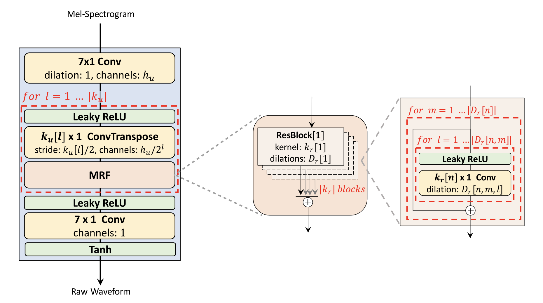
The generator architecture have a few hyper-parameters that can be fine-tuned in a trade-off between synthesis efficiency and sample quality, such as the (hidden dimension $h_{u}$ and kernel sizes $k_{u}$) of the transposed convolutions; and the (kernel sizes $k_{r}$ and dilation rates $D_{r}$) of MRF modules.

Multi-Period Discriminator (MPD)

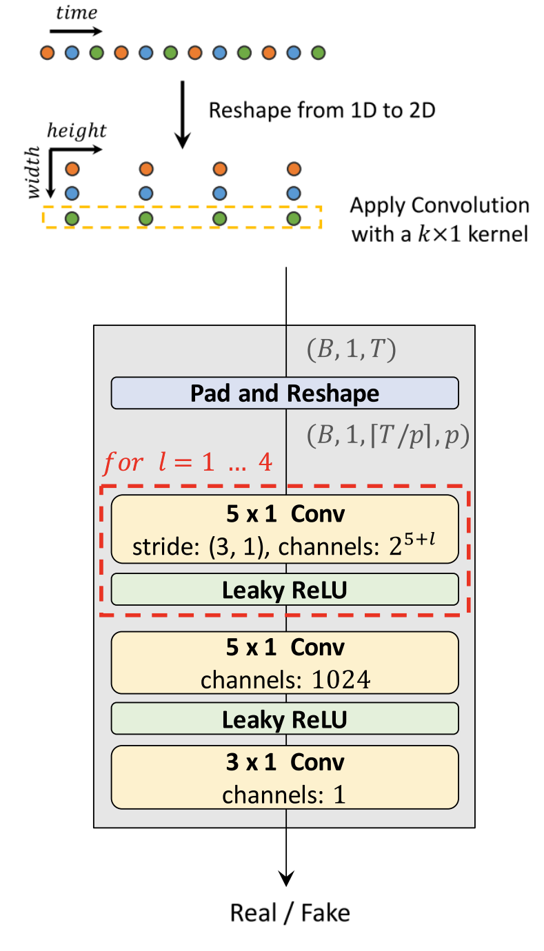
MPD is a mixture of sub-discriminators, each sub-discriminator is a stack of strided convolutional layers with leaky rectified linear unit (ReLU) activation. Sub-discriminator only accepts equally spaced samples of an input audio; the space is given as period $p$. The sub-discriminators are designed to capture different implicit structures from each other by looking at different parts of an input audio. The way MPD works is shown in the following figure:

Given a certain period $p$; in the paper, they set the periods to $\lbrack 2,\ 3,\ 5,\ 7,\ 11\rbrack$ to avoid overlaps as much as possible.
Then, they reshape the 1D raw audio of length $T$ into 2D data of $\left( \frac{T}{p},\ p \right)$
Then, they apply 2D convolutions to the reshaped data, where the kernel size of every convolutional layer is $(k \times 1)$ to process the periodic samples independently on the width axis.
Lastly, weight normalization is applied to MPD.

Multi-Scale Discriminator (MSD)

Because each sub-discriminator in MPD only accepts disjoint samples, they added MSD to consecutively evaluate the audio sequence. The architecture of MSD is drawn from MelGAN, which is a mixture of three sub-discriminators operating on different input scales: raw audio, ×2 average-pooled audio, and ×4 average-pooled audio, as shown in the following figure:

Each of the sub-discriminators in MSD is a stack of strided and grouped convolutional layers with leaky ReLU activation. The discriminator size is increased by reducing stride and adding more layers. Weight normalization is applied except for the first sub-discriminator, which operates on raw audio. Instead, spectral normalization is applied and stabilizes training as it reported.

Note:
MPD operates on disjoint samples of raw waveforms, whereas MSD operates on smoothed waveforms.

GAN Loss

In GAN setup, the discriminator $D$ is trained to classify ground truth samples to 1, and the samples synthesized from the generator $G$ to 0. The generator is trained to fake the discriminator by updating the sample quality to undistinguished from the ground-truth. In the paper, they used a combination of three different losses, which are Adversarial Loss $\mathcal{L}_{Adv}$, Feature Matching Loss $\mathcal{L}_{fm}$, and Mel-spectrogram Loss $\mathcal{L}_{mel}$. The final loss $\mathcal{L}_{G}$ is defined as:

\[\mathcal{L}_{G} = \sum_{k = 1}^{K}{\left\lbrack \mathcal{L}_{Adv}\left( G;D_{k} \right) + \lambda_{fm}\ \mathcal{L}_{fm}\left( G;D_{k} \right) \right\rbrack +}\lambda_{mel}\ \mathcal{L}_{mel}(G)\] \[\mathcal{L}_{D} = \sum_{k = 1}^{K}{\mathcal{L}_{Adv}\left( D_{k};G \right)}\]

Where:

$D_{k}$ denotes the $k$-th sub-discriminator in MPD and MSD.
$\lambda_{fm}$ and $\lambda_{mel}$ are scaling hyper-parameters. In the paper, they set $\lambda_{fm} = 2$ and $\lambda_{mel} = 45$.
The adversarial loss $\mathcal{L}_{Adv}$ is defined as the following; where $x$ denotes the ground truth audio and $s$ denotes the synthesized audio.

\[\mathcal{L}_{Adv}(D;G) = \mathbb{E}_{(x,s)}\left\lbrack \left( D(x) - 1 \right)^{2} + \left( D\left( G(s) \right) \right)^{2} \right\rbrack\] \[\mathcal{L}_{Adv}(G;D) = \mathbb{E}_{s}\left\lbrack \left( D\left( G(s) \right) - 1 \right)^{2} \right\rbrack\]

The Mel-spectrogram Loss $\mathcal{L}_{mel}$ is added to improve the training efficiency of the generator and the fidelity of the generated audio. It is the L1 distance between the mel-spectrogram of a waveform synthesized by the generator and that of a ground truth waveform where is the the function that transforms a waveform into the corresponding mel-spectrogram:

\[\mathcal{L}_{mel}(G) = \mathbb{E}_{(x,s)}\left\lbrack \left\| \phi(x) - \phi\left( G(s) \right) \right\|_{1} \right\rbrack\]

The feature matching $\mathcal{L}_{fm}$ loss is measured by the difference in features of the discriminator between a ground truth sample and a generated sample. Every intermediate feature of the discriminator is extracted, and the L1 distance between a ground truth sample and a conditionally generated sample in each feature space is calculated:

\[\mathcal{L}_{mel}(G;D) = \mathbb{E}_{(x,s)}\left\lbrack {\sum_{i = 1}^{T}{\frac{1}{N_{i}}\left\| D^{i}(x) - D^{i}\left( G(s) \right) \right\|}}_{1} \right\rbrack\]

Such as $T$ denotes the number of layers in the discriminator; $D^{i}$ and $N_{i}$ denote the features and the number of features in the $i$-th layer of the discriminator, respectively.

Experiments

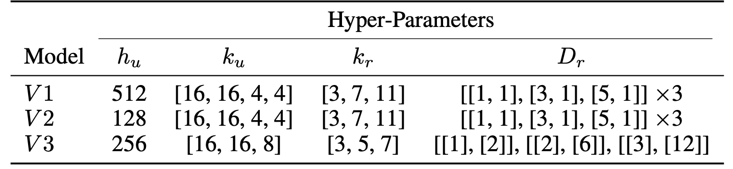
For experiments, they used the LJSpeech dataset which consists of $13,100$ short audio clips of a single speaker with a total length of approximately $24$ hours. The audio format is 16-bit PCM with a sample rate of 22 kHz; it was used without any manipulation. To confirm the trade-off between synthesis efficiency and sample quality, they conducted experiments based on the three variations of the generator, V1, V2, and V 3 while maintaining the same discriminator configuration. The hyper-parameters for these three generators are defined below:

They used 80 bands mel-spectrograms as input conditions. The FFT, window, and hop size were set to $1024$, $1024$, and $256$, respectively. The networks were trained using the AdamW optimizer with $\beta_{1} = 0.9$, $\beta_{2} = 0.99$, and weight decay $\lambda = 0.01$. The learning rate decay was scheduled by a $0.999$ factor in every epoch with an initial learning rate of $2 \times 10^{- 4}$.

Results

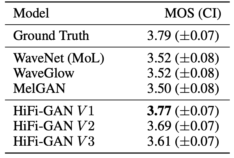
To evaluate the audio quality, the authors crowd-sourced 5-scale MOS tests via Amazon Mechanical Turk. Raters listened to the test samples randomly, where they were allowed to evaluate each audio sample once. All audio clips were normalized to prevent the influence of audio volume differences on the raters. Then, they randomly selected 50 utterances from the LJSpeech dataset and used the ground truth spectrograms of the utterances which were excluded from training as input conditions. Results are reported in the following table:

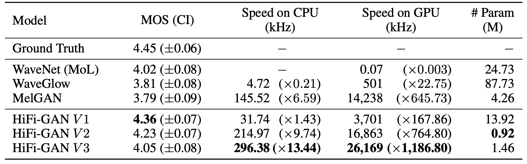
Remarkably, all variations of HiFi-GAN scored higher than the other models. V1 has $13.92M$ parameters and achieves the highest MOS with a gap of $0.09$ compared to the ground truth audio. V2 demonstrates similarity to human quality while significantly reducing the memory requirement and inference time, compared to V1. It only requires $0.92M$ parameters. Despite having the lowest MOS among our models, V3 can synthesize speech $13.44$ times faster than real-time on CPU and $1,186$ times faster than real-time on single V100.

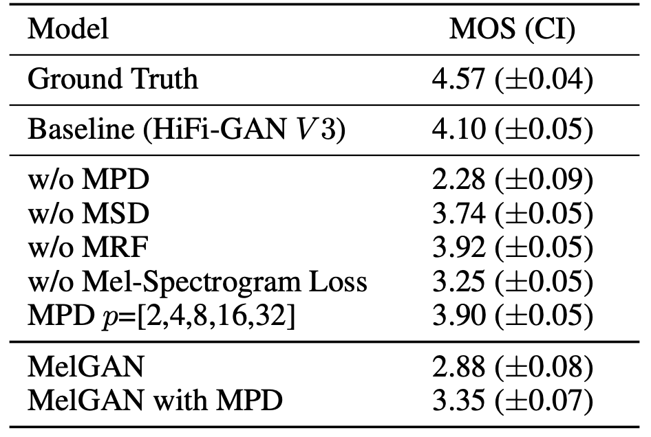
In the paper, they performed an ablation study to verify the effect of each HiFi-GAN component on the quality of the synthesized audio with V3 generator. The results of the MOS evaluation are shown in the following table. Removing MPD causes a significant decrease in audio quality, whereas the absence of MSD shows a relatively small but noticeable degradation. Adding mel-spectrogram loss helps improve the quality. Also, adding MPD to MelGAN shows statistically significant improvement.

To evaluate the generality of HiFi-GAN to the mel-spectrogram inversion of unseen speakers, they used the VCTK multi-speaker dataset, which consists of approximately $44,200$ short audio clips uttered by $109$native English speakers with various accents. The total length of the audio clips is approximately $44$ hours. The audio format is 16-bit PCM with a sample rate of 44 kHz which they reduced to 22 kHz. For evaluation set, they randomly selected nine speakers and excluded all their audio clips from the training set.

The following table shows the results for the mel-spectrogram inversion of the unseen speakers. The three generator were all better than other models, indicating that the proposed models generalize well to unseen speakers.

In the paper, they conducted one last experiment to examine the effectiveness of the proposed models when applied to an end-to-end TTS pipeline. They used this model with Tacotron 2. The results without fine-tuning show that all the proposed models outperform WaveGlow in the end-to-end setting, while the audio quality of all models are below ground-trut. When fine-tuning, V1 achieves better scores. Which means that HiFi-GAN adapts well on the end-to-end setting with fine-tuning.