ConvT-T
ConvT-Transducer stands for “Conv-Transformer Transducer” which is a Transducer-based streamable automatic speech recognition (ASR) system created by Huawei Noah’s Ark Lab in 2020 and published in their paper: Conv-Transformer Transducer: Low Latency, Low Frame Rate, Streamable. The original Transformer architecture, with encoder-decoder architecture, is only suitable for offline ASR as it relies on a bidirectional attention mechanism. To make the Transformer suitable for streaming ASR, they applied the following modifications:
-
They used a unidirectional Transformer which doesn’t require any future context.
-
But future context is important to the speech recognition performance, that’s why they used interleaved convolution layers to model these future context.
-
To reduce computation cost, they gradually downsampled the acoustic input, also with the use of interleaved convolution layers.
-
They limited the length of history context in self-attention to maintain constant computation cost for each decoding step.
Note to the Reader:
A brush-up on the Transducer architecture is much needed before going on with this article.
Architecture
In most of previous works in Transducer framework, transcription network (encoder) and prediction network (decoder) are composed of RNN. However, other types of networks can be used as well. For example, the Conformer paper used Conformer as an encoder and a unidirectional LSTM as a decdoer. Same happens in the ContextNet and T-T papers where they used ContextNet and Transformer as encoders respectively while both used LSTM as a decoder.
In this part, we are going to talk about the three different components of the Conv-Transformer Transducer:
Encoder
In the Conv-Transformer Transducer, the audio encoder is composed of three blocks as shown in the following figure. Each block is composed of three convolution layers followed by unidirectional Transformer. Unidirectional Transformer is similar to encoder of the original Transformer, except that self-attention is masked, preventing the self-attention from attending to subsequent positions beyond current position.

Note:
ConvND-BN-RELU denotes N-Dimensional convolution layers followed by batch normalization and ReLU activation. For convolution layers, $F$ denotes number of filters, $S$ denotes the value of stride, $C$ denotes number of output channels. For Transformer, $L$ denotes number of layers, $N$ denotes number of heads, $\text{DH}$ denotes dimension of each head, $\text{DM}$ denotes input and output dimension of self-attention layers and feed-forward network (FFN) layers, $\text{DF}$ denotes dimension of intermediate hidden layer in the FFN.
As mentioned earlier, the interleaved convolution layers before Transformer in each block. are used to model furture context. In this 3-block setting, the size of look-ahead window is $140\ ms$, which is acceptable in streaming speech recognition. The size of look-ahead window required by current input frame is illustrated in the following figure where input and output of each block are represented by squares, convolution layers are represented by circles, and skipped activations are represented with dashed outline.

Also, they downsampled the input representation with the convolution layers stride. For example, the second convolution layer of each block uses a stride of $2$ along time dimension. With an input frame rate of $10\ ms$, the frame rate becomes $20\ ms$ in the first block, 40 ms in the second block, and finally 80 ms in the third block. According to the paper, this progressive downsampling scheme caused no loss in accuracy.
Decoder
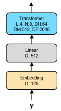
In the Conv-Transformer Transducer, the prediction network (or decoder) is illustrated in the following figure. As shown in the figure, it consists of three blocks:
-
An embedding layer that converts previously predicted non-blank labels into vector representations.
-
A linear layer that projects the embedding vectors to match input dimension of unidirectional Transformer layers.
-
A unidirectional Transformer.

Joint Network
The last network in any Transducer model is the joint network. In this paper, they used a fully-connected feed-forward neural network with single hidden layer. There are 512 units in the hidden layer, with Rectifified Linear Unit (ReLU) as activation function. The outputs of audio encoder and prediction network (decoder) are concatenated and used as input of joint network.
Experiments & Results
Experiments were performed with the LibriSpeech dataset. All the Conv-Transformer Transducer models were trained using NovoGrad as an optimizer. The learning rate is warmed up from $0$ to $0.01$ in the first $10k$ steps, then is decayed to $5 \times 10^{- 6}$ in the following $200k$ steps polynomially. For acoustic features, they used 128-dimensional log-mel filterbank, calculated with $20\ ms$ window and $10\ ms$ stride. For textual features, they used $4k$ subwords generated from training transcripts of LibriSpeech using SentencePiece. To avoid overfitting, they used multiple techiniques:
-
They used additive Gaussian noise.
-
They applied speed perturbation in time domain.
-
They used SpecAugment, but without time-warping (since speed perturbation is already used).
-
Transformer layers are regularized with $10\%$ dropout.
The WER scores of this models with other models on LibriSpeech test-clean and test-other are reported in the following table:

As we can see ConvT-T is achieving the lowest WER on both test-clean and test-other while operating with fewer parameters, smaller look-ahead window, and lower frame rate; compared to other models such as TDNN-LSTM model provided by Kaldi, Transformer Transducer (T-T), a hybrid model with Transformer AM.
Note:
HFR ConvT-T is the same as ConvT-T, the only difference is that it was trained with half the frame rate. ConvT-T was trained on $80\ ms$ frame rate while HFR ConvT-T was trained on $40\ ms$. This was done by setting the stride to 1 instead of 2 in the second convolution layer of the third block. As this model requires more memory, we train the 40-ms model with only half of the original batch size, but with twice more steps to maintain the same number of epochs. As shown in Table 2, the performance difference between the 40-ms model and the 80-ms model is insignificant.
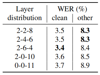
Later in the paper, they performed multiple experiments to analyze effects of varying the number of Transformer layers over different blocks of various frame rates. The results are shown in following table:

They further evaluated the effects of limiting the amount of history context (left-context) in self-attention of Transformer layers. The results are shown in following table:
