FastSpeech

FastSpeech is a novel non-autoregressive Text-to-Speech (TTS) model based on the Transformer architecture. It takes a text (phoneme) sequence as input and generates mel-spectrograms non-autoregressively, later a vocoder is used to convert the spectrogram to audio waveforms. FastSpeech was proposed by Microsoft in 2019 and published in this paper under the same name: “FastSpeech: Fast, Robust and Controllable Text to Speech”. The official synthesized speech samples resulted from FastSpeech can be found in this website. The unofficial PyTorch implementation of FastSpeech can be found in this GitHub repository: FastSpeech.

Architecture

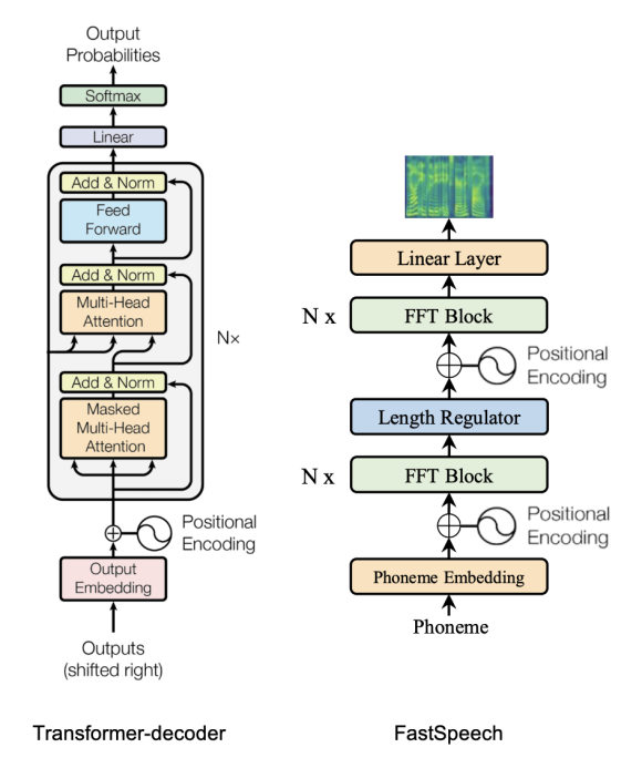
Since a mel-spectrogram sequence is much longer than its corresponding phoneme sequence, FastSpeech adopts a Length Regulator that up-samples the phoneme sequence according to the phoneme duration (i.e., the number of mel-spectrograms that each phoneme corresponds to) to match the length of the mel-spectrogram sequence. The Length Regulator is built on a phoneme duration predictor, which predicts the duration of each phoneme. The whole architecture of FastSpeech is shown below:

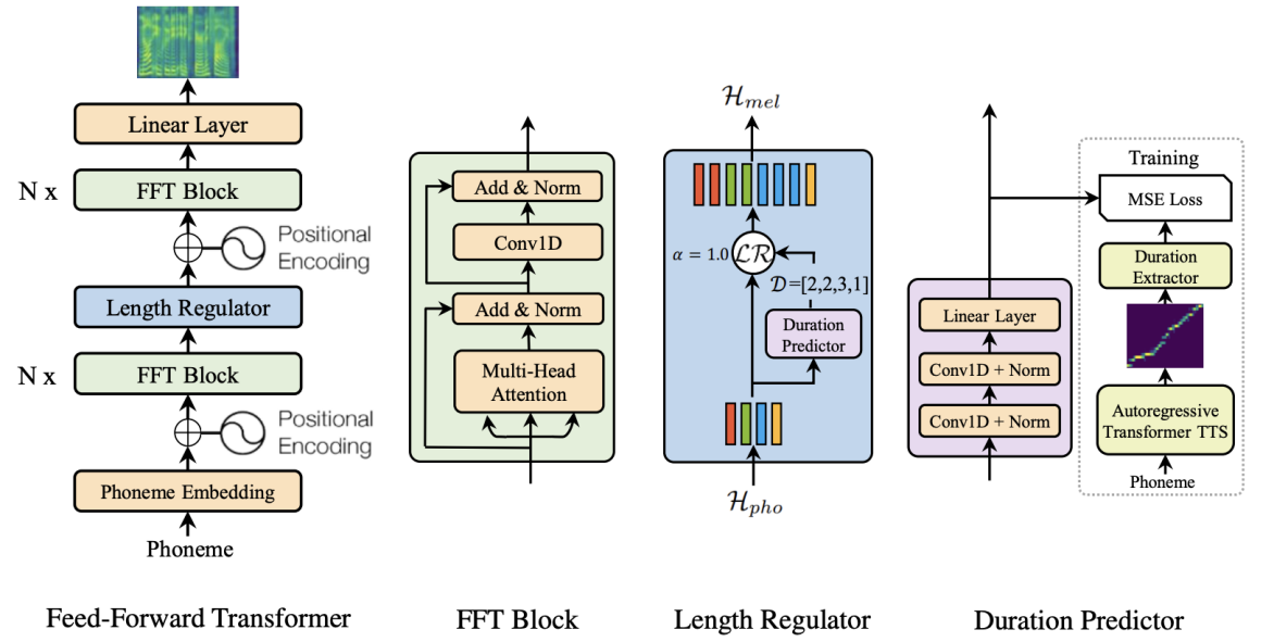
From the previous figure, we can see that FastSpeech consists of three main components: Feed-forward Transformer, Duration Predictor, and Length Regulator. In the next part, we are going to talk about each component in more details.

Feed-forward Transformer

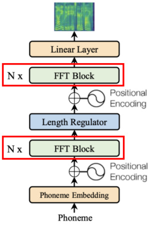
Feed-Forward Transformer, highlighted in red box in the following figure, stacks multiple FFT blocks for phoneme to mel-spectrogram transformation, with $N$ blocks on the phoneme side, and $N$ blocks on the mel-spectrogram side, with a Length Regulator (which will be described in the next subsection) in between to bridge the length gap between the phoneme and mel-spectrogram sequence.

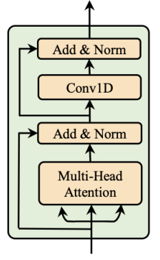
Each FFT block, as shown below, consists of multi-head self-attention mechanism to extract the cross-position information and 2-layer 1D convolutional network with ReLU activation instead of the dense network in Transformer. The motivation is that the adjacent hidden states are more closely related in the character/phoneme and mel-spectrogram sequence in speech tasks. Similar to Transformer, residual connections, layer normalization, and dropout are added after the self-attention network and 1D convolutional network respectively.

Note:
The Feed-forward Transformer on the phoneme side is usually referred to as the “Encoder” while the one on the mel-spectrogram side is referred to as the “Decoder”.

Length Regulator

The Length Regulator is used to solve the problem of length mismatch between the phoneme and spectrogram sequence in the Feed-Forward Transformer. As said earlier, the mel-spectrogram sequence is expected to be way longer then the phoneme sequence. And to solve this problem, the Length Regulator expands the hidden state of the phoneme sequence so it equals the length of the mel-spectrogram sequence.

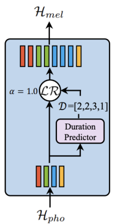
More formally, given phoneme sequence hidden states as $H_{pho} = \left\lbrack h_{1},\ h_{2},…h_{n} \right\rbrack$, where $n$ is the length of the phoneme sequence. And the phoneme duration (how many mel-spectrogram frames for each phoneme) sequence as $D = \left\lbrack d_{1},\ d_{2},…d_{n} \right\rbrack$, where $\sum_{i = 1}^{n}d_{i} = m$ and $m$ is the length of the mel-spectrogram sequence and $m \gg n$. The Length Regulator $LR$ expands $H_{pho}$ to become $H_{mel}$ according to the following formula where $\alpha$ is a hyper-parameter:

\[H_{mel} = LR\left( H_{pho},\ D,\ \alpha \right)\]

For example, given $H_{pho} = \left\lbrack h_{1},\ h_{2},\ h_{3},\ h_{4} \right\rbrack$ and $D = \lbrack 2,\ 2,\ 3,\ 1\rbrack$, the expanded sequence $H_{mel}$ becomes $\left\lbrack h_{1},\ h_{1},\ h_{2},\ h_{2},\ h_{3},\ h_{3},\ h_{3},\ h_{4} \right\rbrack$. As you can see, phoneme $h_{1}$ was repeated twice since the duration predictor predicted $2$, same happens for phoneme $h_{2}$ ...etc. Now, the phoneme sequence (whose previous length was $n$) is equal to the mel-spectrogram sequence with a length of $m$.

In the previous case, $\alpha = 1$ which is the normal speed. When $\alpha = 1.3$ (slow speed) or $\alpha = 0.5$ (fast speed), the duration sequences become $D_{\alpha = 1.3} = \lbrack 2.6,\ 2.6,\ 3.9,\ 1.3\rbrack \approx \lbrack 3,\ 3,\ 4,\ 1\rbrack$ and $D_{\alpha = 0.5} = \lbrack 1,\ 1,\ 1.5,\ 0.5\rbrack \approx \lbrack 1,\ 1,\ 2,\ 1\rbrack$, respectively. As you might predicted, the Length Regulator $LR$ can easily adjust voice speed by lengthening or shortening the phoneme duration.

Note:
The Length Regulator $LR$ can also control the break between words by adjusting the duration of the space characters in the sentence, so as to adjust part of prosody of the synthesized speech

At this point, we discussed how the Length Regulator $LR$ uses phoneme duration $D$ to regularize the sequence length difference. In the next part, we are going to talk about how to predict $D$ in the first place.

Duration Predictor

In the paper, they refer to the phoneme duration $D$ as the number of mel-spectrogram frames that maps to each phoneme. So, $D = \lbrack 2,\ 2,\ 3,\ 1\rbrack$ means that the first and second phonemes map to two mel-spectrogram frames each, and the third phoneme maps to three frames while the last phoneme maps to just one frame. As you have seen earlier, this sequence is very important to the Length Regulator. Here, we are going to discuss how eht authors predicted this $D$ sequence.

Duration Predictor module, as shown in the following figure, consists of a 2-layer 1D convolutional network with ReLU activation, each followed by the layer normalization and the dropout layer, and an extra linear layer to output a scalar, which is exactly the predicted phoneme duration.

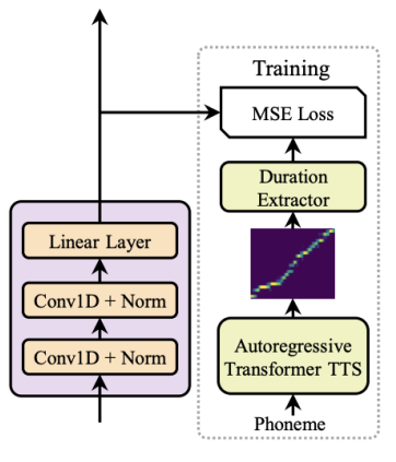
The Duration Predictor is only used in the inference phase. During the training phase, the ground-truth phoneme duration are extracted from an autoregressive teacher TTS model, as shown in the previous figure. The following is the detailed steps:

First, they train an auto-regressive teacher TTS model. In the paper, they used Transformer TTS model.
For each training sequence pair, they extract the decoder-to-encoder attention alignments from the trained teacher model. Since there are multiple attention alignments (one for each head), they compute a focus rate $F$ (defined below) for each head and choose the one with the highest focus.

\[F = \frac{1}{S}\sum_{s = 1}^{S}{\max_{1 \leq t \leq T}a_{s,t}}\]

Where $S$ and $T$ are the lengths of the ground-truth spectrograms and phonemes, as, $a_{s,t}$ donates the element in the $s$-th row and $t$-th column of the attention matrix. The following figure shows the different between a good alignment (has higher focus) and a bad alignment (has lower focus):

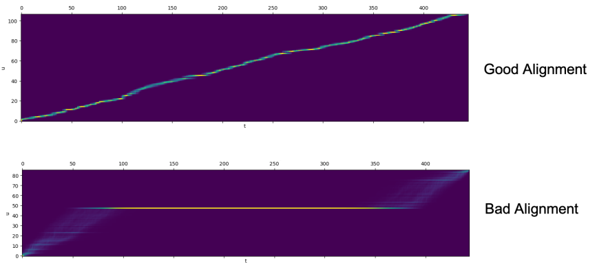
Finally, the phoneme duration sequence $D$ is the number of mel-spectrograms attended to each phoneme according to the attention matrix selected in the above step. Now, the phoneme duration sequence is defined as:

\[d_{i} = \sum_{s = 1}^{S}\left\lbrack \underset{t}{\arg\max}a_{s,t} = i \right\rbrack\]

Experiments

Regarding dataset, in this paper they used LJSpeech dataset, which contains $13,100$ English audio clips and the corresponding text transcripts, with the total audio length of approximate 24 hours. Dataset was randomly split into 3 sets: $12500$ samples for training, $300$ samples for validation and $300$ samples for testing.

Regarding text pre-processing, they converted the text sequence into the phoneme sequence using grapheme-to-phoneme (g2p) tool. Regarding audio pre-processing, they converted the raw waveform into mel-spectrograms using frame size of $1024$ and hop size of $256$.

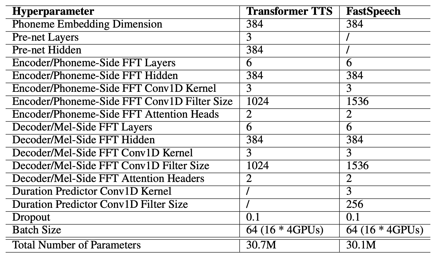
Regarding the architecture, FastSpeech consisted of $6$ FFT blocks on both the phoneme side and the mel-spectrogram side. The size of the phoneme vocabulary was $51$, including punctuations. The dimension of phoneme embeddings, the hidden size of the self-attention and 1D convolution in the FFT block were all set to $384$. The number of attention heads was set to $2$. The kernel sizes of the 1D convolution in the 2-layer convolutional network were both set to $3$, with input/output size of $384/1536$ for the first layer and $1536/384$ in the second layer. The output linear layer converts the $384$-dimensional hidden into $80$-dimensional mel-spectrogram.

Regarding the duration predictor, the kernel sizes of the 1D convolution were set to $3$, with input/output sizes of $384/384$ for both layers. The teacher TTS had the same configuration as Transformer TTS, which consists of a 6-layer encoder, a 6-layer decoder, except that they used 1D convolution network instead of position-wise FFN. This teach model was trained with batch size of $16$ sentences with Adam optimizer with $\beta_{1} = 0.9$, $\beta_{2} = 0.98$, and $\epsilon = 10^{- 9}$. It takes $80k$ steps for training until convergence.

Note:
In this paper, the teacher model serves two purposes:

To extract the phoneme duration as the target to train the duration predictor.

To perform sentence-level knowledge distillation. This is how it works: given a source text sequence, they used the teacher model to generate the mel-spectrograms creating new paired data that can be used for FastSpeech model further training.

The complete list of hyper-parameters used to train FastSpeech and the teacher model (Transformer TTS) is shown below:

Results

In this part, we are going to discuss the performance of FastSpeech in terms of:

Audio Quality:
They compared FastSpeech to the ground-truth with/without Vocoder, Tacotron 2, Merlin (popular parametric TTS), and Transformer TTS. All previous models used WaveGlow as vocoder except Merlin used WORLD Vocoder. The results are shown in the following table which shows that FastSpeech can nearly match the quality of the Transformer TTS and Tacotron 2 models.

Inference Speedup:
They compared the inference of FastSpeech compared with Transformer TTS model, which has similar number of model parameters and results are shown in the following table. Without Vocoder, FastSpeech speeds up the mel-spectrogram generation by $269.40$x. With Vocoder, FastSpeech still achieves $38.30$x speedup for audio generation.

As an ablation study to verify the effectiveness of several components in FastSpeech, including 1D Convolution and sequence-level knowledge distillation, they performed some experiments and reported the results in the following table; which shows how much important is the sentence-level knowledge distillation.