Transformer TTS

Transformer TTS is a non-autoregressive TTS system that combines the advantages of Tacotron 2 and Transformer in one model, in which the multi-head attention mechanism is introduced to replace the RNN structures in the encoder and decoder, as well as the vanilla attention network. Transformer TTS was proposed by Microsoft in 2018 and published in this paper: “Neural Speech Synthesis with Transformer Network”. The official audio samples resulted from this model can be found in website. The unofficial PyTorch implementation of this paper can be found in this GitHub repository: Transformer-TTS.

Recent end-to-end neural text-to-speech (TTS) models such as Tacotron and Tacotron 2 depend intensively on recurrent neural networks (RNNs) which are very slow to train and can’t capture long dependencies. That’s why Transformer TTS model was proposed. In this model, they adapted the multi-head attention mechanism from Transformer to replace the RNN structures and the original attention mechanism in Tacotron 2.

Architecture

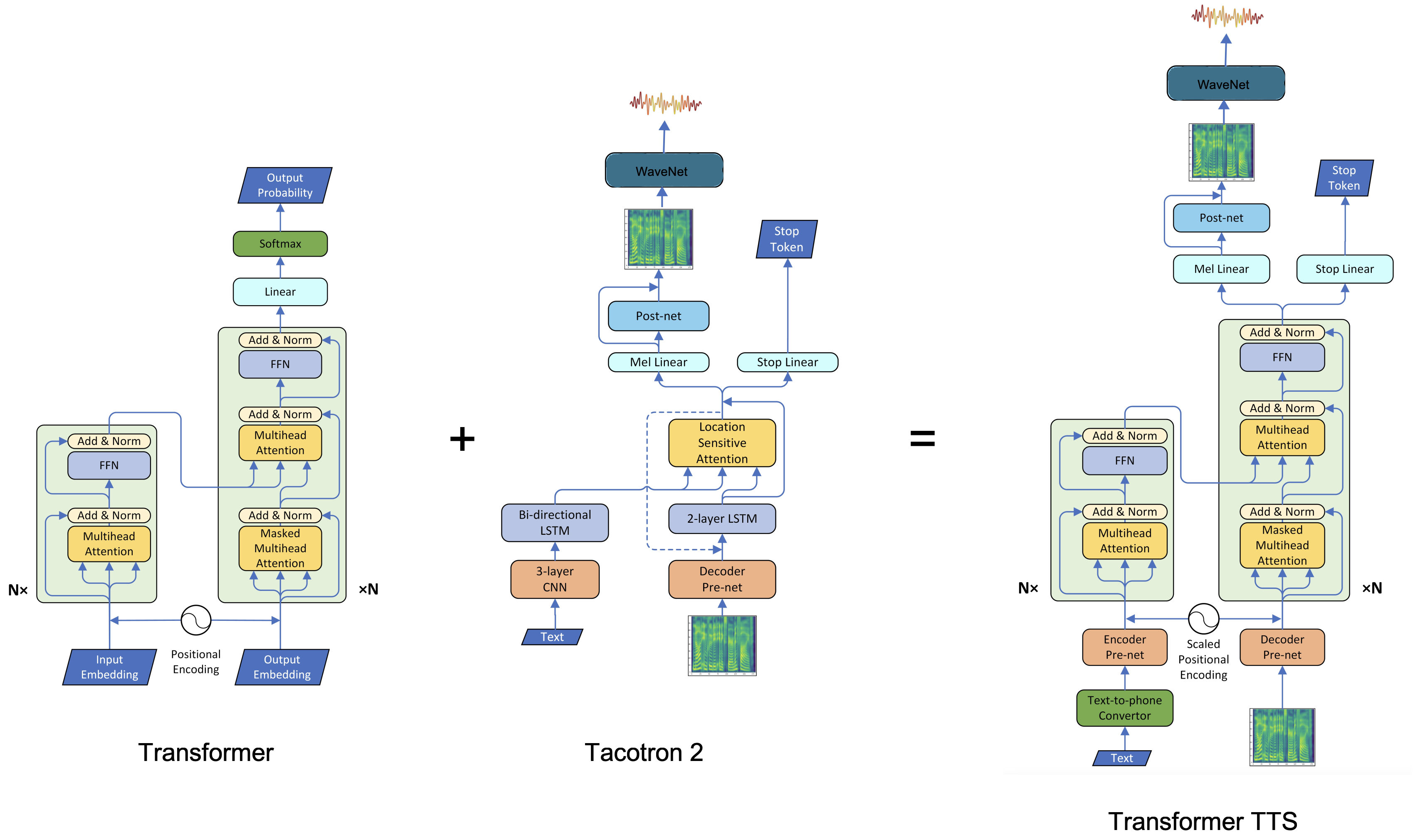
The architecture for Transformer TTS can be seen in the following figure which shows that Transformer TTS consists of five different components: Text-to-phone Converter, Encoder, Decoder, Post-network, and Vocoder. The encoder and decoder networks have additional components added to them called “encoder per-net” and “decoder pre-net” respectively.

In the next part, we are going to discuss the different parts of Transformer-TTS in more details.

Text-to-phone Converter

In Transformer TTS model, they decided to convert input text to phonemes. If you don’t know, a phoneme is a distinct unit of sound in a specified language. For example, the letter “a” in English has multiple different phonemes (“eı”, “æ”, “a:”), each sounds different even though it originates from the same letter. In this model, they used trainable embedding of $512$ dims. Also, note that word boundaries and punctuations are included in this module as special markers.

Scaled Positional Encoding

In the Transformer paper, they implemented positional encoding to take the order of the input sequence into consideration. This was done by injecting information about the relative or absolute position of frames by positional embeddings, shown in the following equation:

Where $\text{pos}$ is the word position/index (starting from zero). $i$ is the $i^{\text{th}}$ value of the word embedding and $d$ is the size of the word embedding. So, if $i$ is even, then we are going to apply the first equation; and if $i$ is odd, then we are going to apply the second equation. After getting the positional vectors, we add them to the original embedding vector to get context vector:

Since the source domain is of texts while the target domain is of mel-spectrograms, hence using fixed positional embeddings may impose heavy constraints on both the encoder and decoder pre-nets. That’s why they decided to use a trainable weight $\alpha$, so that these embedding can adaptively fit the scales of both encoder and decoder prenets’ output, as shown in the following equation:

Where $\text{prenet}$ is either the encoder or the decoder prenet, $\text{ph}_{i}$ is the phoneme at position $i$, $\text{PE}$ is the positional embedding, and $\alpha$ is the trainable weight.

Encoder

The encoder part of the Transformer TTS model is the same as the encoder in the Transformer model consisting of 6 layers. The only difference here is the “pre-network”. The goal of the pre-network here is to extract contextual features from the input phoneme embeddings, which can be used in further steps to train the encoder architecture.

The pre-network they used here is the same pre-network in the Tacotron 2, which is a 3-layer CNN applied to the input phoneme embeddings. Each convolution layer has 512 channels, followed by a batch normalization and ReLU activation, and a dropout layer as well. In addition, they added a linear projection after the final ReLU activation, to reduce the effect of ReLU on the embeddings.

Remember, the output range of ReLU is $\lbrack 0,\ + \infty)$, while each dimension of these embeddings is in $\left\lbrack - 1,1 \right\rbrack$. Adding 0-centered positional information onto non-negative embeddings will result in a fluctuation not centered on the origin and harm model performance. Hence they added a linear projection for center consistency.

Decoder

The decoder part of the Transformer TTS model is the same as the decoder in the Transformer model, cosisting of 6 layers. The only difference here is the “pre-network”. The goal of the pre-network here is to project the mel-spectrograms into the same subspace as phoneme embeddings, so that the similarity of a encoder embeddings and decoder embeddings can be measured, thus the attention mechanism can work.

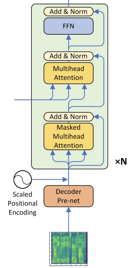
The pre-network they used here is basically two fully connected layers, each has $256$ hidden units with ReLU activation. However, in the paper they tried also $512$ but didn’t improve the performance. An additional linear projection is also added after the ReLU not only for center consistency (like encoder pre-network) but also obtain the same dimension as the positional embeddings whose dimension is $512$.

Post-network

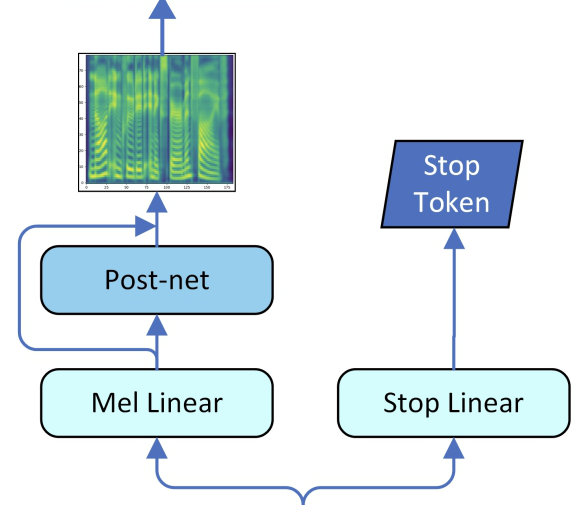
Same as Tacotron 2, they used two different linear projections to predict the mel-spectrogram and the stop token respectively, and used a 5-layer CNN to produce a residual to refine the reconstruction of mel spectrogram.

It’s worth mentioning that, for the stop linear, there is only one positive sample in the end of each sequence which means “stop”, while hundreds of negative samples for other frames. This imbalance may result in unstoppable inference. To fix that, they imposed a positive weight $\left( 5.0 \sim 8.0 \right)$ on the tail positive stop token when calculating binary cross entropy loss, and this problem was efficiently solved.

Vocoder

They used WaveNet to convert mel-spectrogram into audio waveforms. Instead of using 30 layers of dilated convolution, they used 2 layers of Quasi-RNN layers + 20 dilated convolution layers; and the sizes of all residual channels and dilation channels are all 256. Each frame of QRNN’s final output is copied 200 times to have the same spatial resolution as audio samples and be conditions of 20 dilated layers.

This model was trained on mel-spectrogram from the internal US English female dataset, the same dataset used for the TTS training. The sample rate of ground truth audios is $16000$ and frame rate of ground truth mel-spectrogram is $80$.

Experiments

To train the Transformer TTS model, they used an internal US English female dataset, which contains 25-hour professional speech (17584 text-audio pairs), with a few too long waves removed). $50\ \text{ms}$ silence at head and $100\ \text{ms}$ silence at tail are kept for each wave.

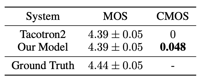
Regarding evaluation, they randomly select 38 fixed examples outside the training set with various lengths as the evaluation set. They used Mean Option Score (MOS) where each audio is listened to by at least 20 testers, who are all native English speakers. To better compare the audio naturalness between Transformer TTS and Tacotron 2, they used Comparison MOS (CMOS) where testers listen to two audios (generated by the two models with the same text) each time and evaluates how the latter feels comparing to the former using a score in $\left\lbrack - 3,3 \right\rbrack$ with intervals of $1$. The order of the two audios changes randomly. Results are shown in the following table

Ablation Study

In this section, we will discuss the different modifications they tried to experiment on the Transformer TTS model and show the performance:

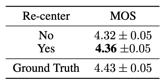
• As discussed in the encoder/decoder pre-network part, they used a linear layer to for consistent center. They experimented with keeping and removing this part and the results show that keeping this linear layer performs slightly better:

• As discussed in the scaled positional embedding part, they added a trainable weight $\alpha$. The results show that keeping this trainable weight performs better.

• The Transformer TTS uses 6 layers on both the encoder and decoder side. They experimented reducing it to 3 and the results show that 6 is better:

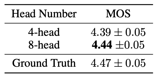
• The Transformer TTS uses 8 attention heads. They experimented reducing it to 4 and the results show that 8 is better: