Glow-TTS

Glow-TTS, a flow-based generative non-autoregressive model for two-staged Text-to-Speech systems. Given an input text, Glow-TTS is able to generate mel-spectrogram that does not require any external aligner, unlike other models such as FastSpeech or ParaNet. Glow-TTS model was proposed by Kakao Enterprise and published in this paper under the same name: “Glow-TTS: A Generative Flow for Text-to-Speech via Monotonic Alignment Search”. The official implementation of this model can be found in this GitHub repository: glow-tts. The official synthetic audio samples resulting from Glow-TTS can be found in this website.

Note:
Glow-TTS is inspired by Glow (a flow-based generative model created by OpenAI in 2018), hence the name.

Note to Reader:
Before going on with this post, I really urge you to check the “Generative Models Recap” part in the WaveGlow post. In this part, you will know more about flow-based generative models such as Glow.

Glow-TTS combines the properties of flow-based models and dynamic programming to efficiently search for the most probable monotonic alignment between text and the latent representation of speech. Enforcing hard monotonic alignments enables the model to generalize to long utterances, and employing flows enables fast, and controllable speech synthesis. By altering the latent representation of speech, they were able to synthesize speech with various intonation patterns and regulate the pitch of speech. Also, Glow-TTS can be extended to a multi-speaker setting with only a few modifications.

Architecture

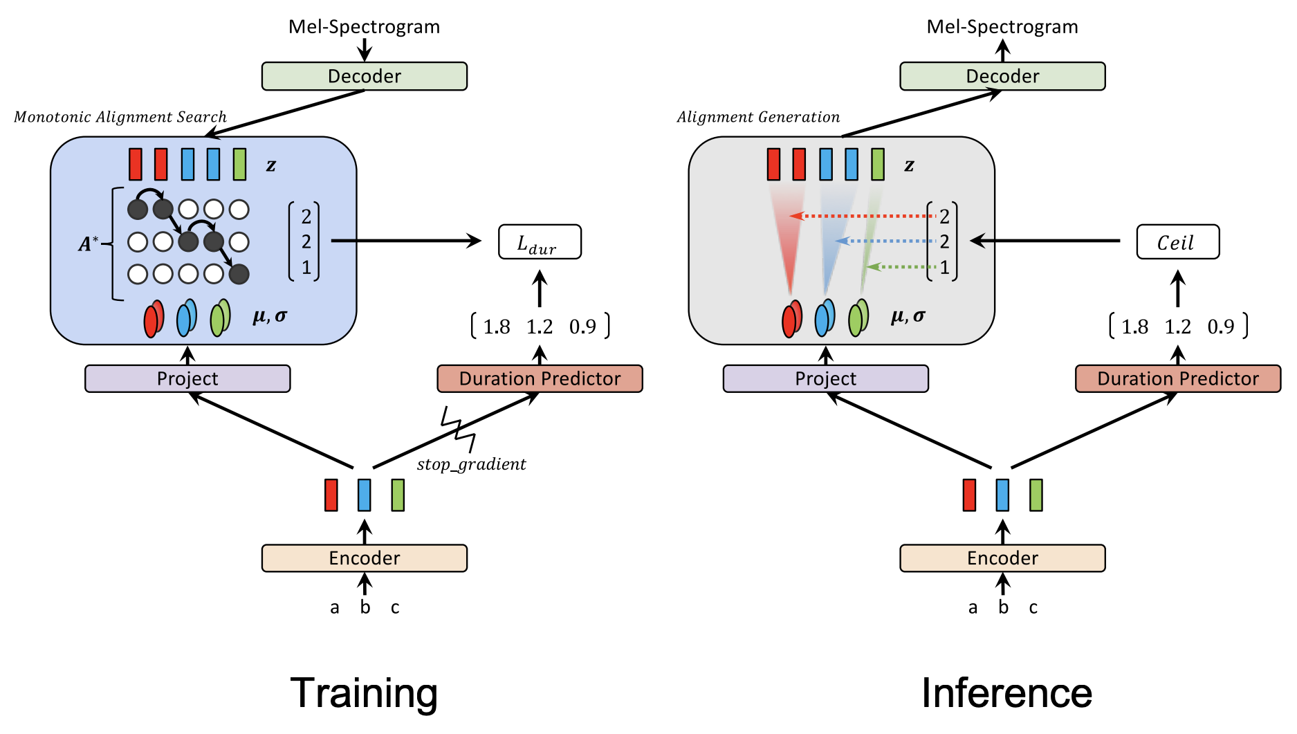
The overall architecture of Glow-TTS is shown in the following figure. The Encoder gets a text sequence and processes it resulting in hidden representation $h$, which is passed to two modules: a linear projection layer to estimate the (mean, covariance) of the prior distribution and a Duration Predictor network to predict the duration. During training, the Decoder efficiently transforms a mel-spectrogram into the latent representation. Then, the Monotonic Alignment Search (MAS) algorithm tries to align the encoder’s prior distribution to the decoder’s latent representation. During inference, the Decoder (being a flow-based model) reverses its role and transforms the aligned representation to mel-spectrogram.

Given a text $c$ and mel-spectrogram $x$, Glow-TTS tries to model the conditional distribution of mel-spectrograms $P\left( x \middle| c \right)$. Glow-TTS does that by transforming the past conditional distribution to another conditional prior distribution $P\left( z \middle| c \right)$ using transformation function $f$ as shown in the following equation:

Where $P\left( x \middle| c \right)$ is a distribution of mel-spectrogram $x$ conditioned on text $c$, $P\left( z \middle| c \right)$ is a prior distribution of latent representation $z$ conditioned on text $c$ which is the task of the Encoder. The $\left| det\ \frac{\partial f^{- 1}(x)}{\partial x} \right|$ term is basically a scaling number, which is the determinant of the Jacobian matrix of the transformation function $f$. This transformation function should be able to transform latent representation $z$ to mel-spectrogram $x$, which is the job of the decoder.

Encoder

Glow-TTS encoder, shown in the following figure, follows the encoder structure of Transformer TTS with two main difference:

• They removed the positional encoding and add relative position representations into the self-attention modules instead

• They also added residual connections to the encoder pre-net.

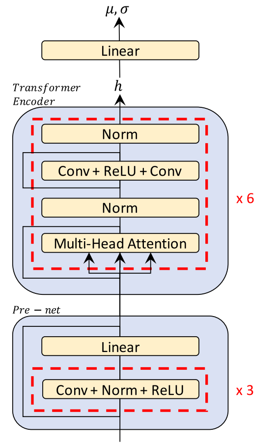
The encoder maps input text $c = c_{1:T}$ where $T$ is the text length into latent representation $h$ which is consecutively passed to a one-linear projection layer in order to estimate the mean $\mu = \mu_{1:T}$ and covariance $\sigma = \sigma_{1:T}$ of the prior distribution, which is multivariate Gaussian distribution. And the same latent representation $h$ is passed to another module called “Duration Predictor”.

Duration Predictor

The duration predictor architecture and configuration is the same as those of FastSpeech, which is composed of two convolutional layers with ReLU activation, layer normalization, and dropout followed by a projection layer.

The duration predictor is trained with the mean squared error loss (MSE) in the logarithmic domain as shown in the following equation:

Where:

• $T_{text}$ and $T_{mel}$ are the length of the input text and mel-spectrogram respectively.

• $d_{i}$ is the duration for the $i^{th}$ character/phoneme in the input text.

• $A^{\ast}$ is the most probable alignment, resulting from MAS.

• $f_{dur}$ is the duration predictor.

• $h$ is the encoder latent representation.

• $sg\lbrack.\rbrack$ is the stop-gradient operator, which removes the gradient of input in the backward pass.

Note:
The duration predictor used here is deterministic, which means that it will produce the same duration given the same input.

Monotonic Alignment Search (MAS)

MAS searches for the most probable monotonic alignment between the latent representation $z_{1:T_{mel}}$ resulting from the decoder during training; and the statistics of the prior distribution $\left( \mu_{1:T_{text}},\sigma_{1:T_{text}} \right)$ resulting from the encoder + projection layer. The Monotonic Alignment Search (MSA) algorithm can be see down below:

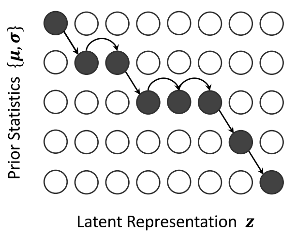
Inspired by the fact that a human reads out text in order, this algorithm enforces hard monotonic alignments. Monotonic alignment means that the alignment between the two variables are not decreasing at any point. For example, the following figure shows an example of possible monotonic alignments. As you can see, the alignment (denoted by dark circles) are either going to the right or down side, never up or to the left side.

Decoder

The core part of Glow-TTS is the flow-based decoder that has similar structure as Glow. It consists of a stack of 12 blocks, each of which consists of an activation normalization layer (ActNorm), invertible $1 \times 1$ convolution layer, and affine coupling layer. The affine coupling layer architecture used here is inspired by WaveGlow except for that they didn’t use the local conditioning.

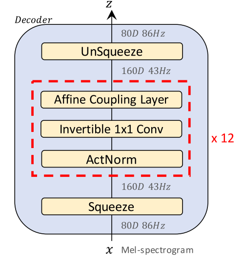
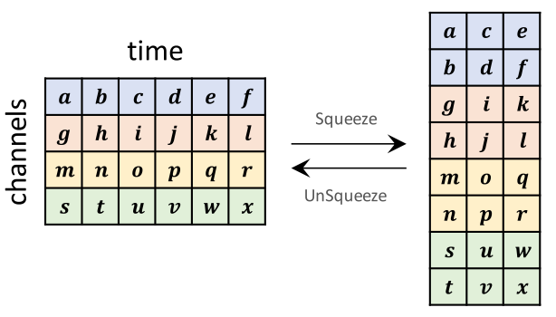
The decoder gets a mel-spectrogram as input and squeezes it. When squeezing, the channel size doubles up and the number of time steps becomes a half. If the number of time steps is odd, they simply ignore the last element. After the data runs over all the 12 blocks, the model un-squeezes it back to the original shape.

Experiments & Results

To evaluate the proposed methods, they conducted experiments on LJSpeech, which consists of $13,100$ short audio clips with a total duration of approximately $24$ hours. They randomly split the dataset into the training set ($12,500$ samples), validation set ($100$ samples), and test set ($500$ samples).

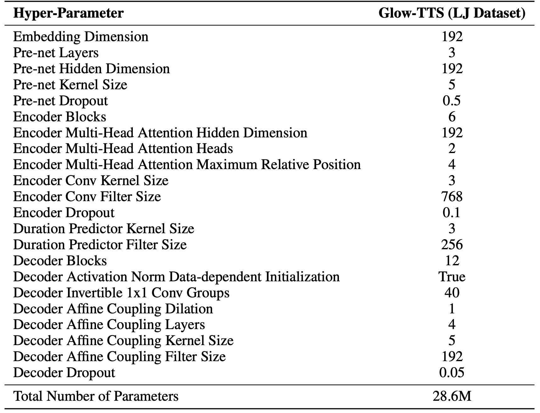
For all the experiments, phonemes were chosen as input text tokens and WaveGlow was used a vocoder. Glow-TTS was trained for $240K$ iterations using the Adam optimizer with the Noam learning rate schedule. The full list of hyper-parameters used to train Glow-TTS can be found in the following table:

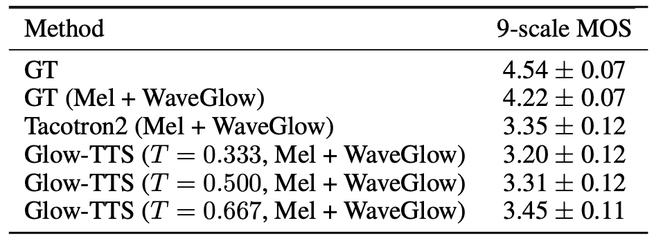
To measure the quality of Glow-TTS, they measured the mean opinion score (MOS) via Amazon Mechanical Turk, including ground truth (GT), and the synthesized samples; 50 sentences are randomly chosen from the test set for the evaluation. The results are shown in the following table:

As you can see from the table, the quality of speech converted from the GT mel-spectrograms by the vocoder ($4.19 \pm 0.07$) is the upper limit of the TTS models. They varied the standard deviation (i.e., temperature $T$) of the prior distribution at inference; Glow-TTS shows the best performance at the temperature of $T = 0.333$.

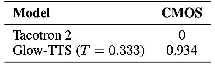
Additionally, they conducted 7-point CMOS evaluation between Tacotron 2 and Glow-TTS with the sampling temperature $\sigma = 0.333$. Through 500 ratings on 50 items, Glow-TTS wins Tacotron 2 by a gap of $0.934$ as shown in the following table:

Controllability

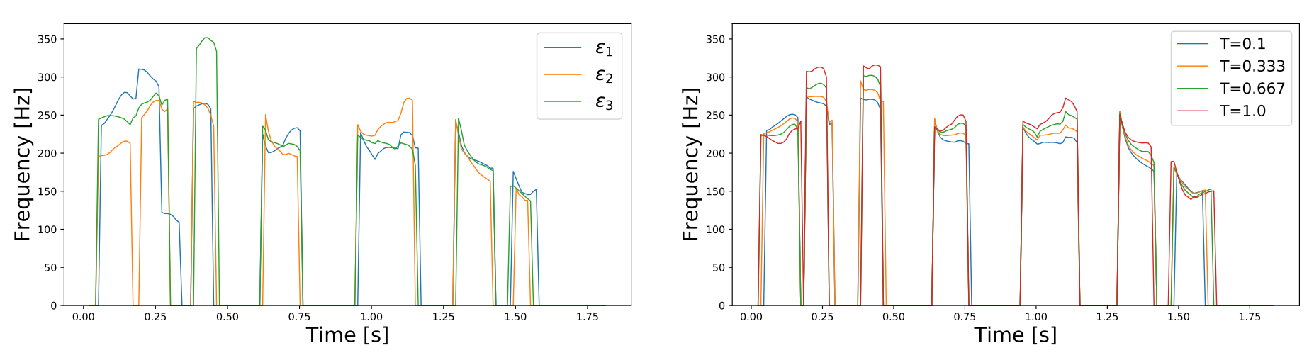
Because Glow-TTS is a flow-based generative model, it can synthesize diverse samples; each latent representation $z\sim\mathcal{N}(\mu,\sigma)$ sampled from an input text is converted to a different mel-spectrogram $f_{dec}(z)$ according to the following expression where $\epsilon$ is a random Gaussian noise:

To decompose the effect of $\epsilon$ and $\sigma$, they experimented with changing them on at a time. They found out that $\epsilon$ controls the intonation patterns of speech while $\sigma$ controls the pitch of speech. The following two figures show the pitch tracks of the same sentence. The one on the right has same temperature $\sigma = 0.667$ with different Gaussian noise $\epsilon$, while the one on the left has the same Gaussian noise $\epsilon$ and different temperature.

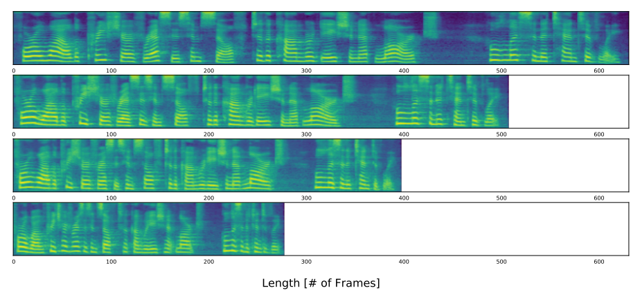
Additionally, they will able to control the speech speed by multiplying a positive scalar value across the predicted duration of the duration predictor. The following figure shows resulting spectrogram with different speech speed obtained by multiplying predicted duration by $1.25$, $1.0$, $0.75$, and $0.5$ respectively:

Multi-speaker Experiments

For the multi-speaker setting, they experimented Glow-TTS with the train-clean-100 subset of the LibriTTS corpus, which consists of audio recordings of 247 speakers with a total duration of about 54 hours. First, they trimmed the beginning and ending silence of all the audio clips and filtered out the data with text lengths over $190$. Then, they split it into the training ($29,181$ samples), validation ($88$ samples), and test sets ($442$ samples).

To train multi-speaker Glow-TTS, they added the speaker embedding and increased the hidden dimension. The speaker embedding is applied in all affine coupling layers of the decoder as a global conditioning. The rest of the settings are the same as for the single speaker setting. For comparison, they also trained Tacotron 2 as a baseline, which concatenates the speaker embedding with the encoder output at each time step. All multi-speaker models were trained for $960K$ iterations.

They measures the MOS as done in single-speaker experiments. However, they used one utterance per speaker, and they chose 50 different speakers randomly. The results are presented in the following table which shows that Glow-TTS achieves comparable quality to Tacotron 2: