Wave-Tacotron

Wave-Tacotron is a single-stage end-to-end Text-to-Speech (TTS) system that directly generates speech waveforms from text inputs. Wave-Tacotron was proposed by Google Research in 2020 and published in this paper under the same name: “Wave-Tacotron: Spectrogram-free end-to-end text-to-speech synthesis”. The official audio samples from Wave-Tacotron can be found in this website. Sadly, I couldn’t find any public implementation for this paper.

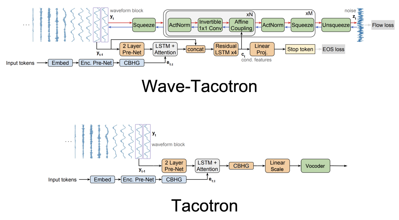
Wave-Tacotron got its name from extending the Tacotron model by integrating a normalizing flow-based vocoder into the auto-regressive decoder. As you can see from the following figure, Wave-Tacotron uses almost the same Encoder & Decoder as Tacotron with minor modifications to the decoder that we will talk about later; and it uses a Normalizing Flow module instead of the Vocoder for the waveform generation part.

Recent work, such as FastSpeech 2 and EATS, has integrated normalizing flows with sequence-to-sequence TTS models, to directly generate waveforms, but they rely on spectral losses and mel spectrograms for alignment. In contrast, Wave-Tacotron avoids spectrogram generation altogether and use a normalizing flow to directly model time-domain waveforms, in a fully end-to-end approach, simply maximizing likelihood.

Architecture

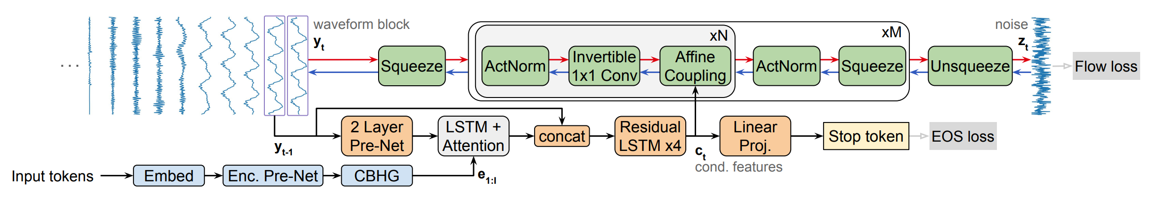
Wave-Tacotron architecture consists of three main components as shown in the following figure: Text Encoder (blue, bottom), Decoder (orange, center) and Normalizing Flow (green, top). The text encoder encodes the $I$-long (character or phoneme) embeddings $x_{1:I}$ to latent representations $e_{1:I}$, which is passed to the decoder to produce conditioning features $c_{t}$ for each output step $t$.

During training (red arrows), the normalizing flow converts these features to noise $z_{t}\sim\mathcal{N}(0,1)$ sampled from a normal distribution. During generation (blue arrows), the flow-inverse is used to generate waveforms $y_{t} \in \mathbb{R}^{K}$ from a random noise sample where $K = 960$ at a $24\ kHz$ sample rate. The model is trained by maximizing the likelihood using the flow and EOS (end-of-sentence) losses (gray).

Note:
Flow-based networks are reversible, which means that you can train a flow-based network on a certain task and be able to perform the reverse of that task without the need of additional training.

In the following sections, we are going to talk about the three main components of Wave-Tacotron in more details:

Text Encoder

Similar to the Tacotron model, the text encoder in Wave-Tacotron tries to extract robust sequential representations from phoneme or character sequence. The encoder consists of three main modules:

• The embedding layer which converts the one-hot embedding for the phoneme or character sequence to embeddings.

• Each of these character emeddings is passed to the “pre-net” block which is basically a non-linear bottleneck layer with dropout.

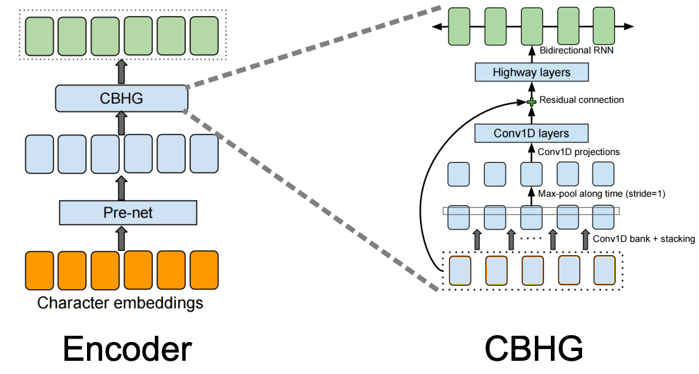
• Finally, the output from the pre-net is passed to the CBHG (Convolution Bank + Highway GRU) network which transforms the pre-net outputs into the final encoder representation. The CBHG network consists of a bank of 1-D convolutional filters, followed by highway networks and a bidirectional GRU layer.

The following figure shows the architecture for the encoder and the CBHG network:

Decoder

The decoder is very similar to the one used in Tacotron with the following minor modifications:

• They used location-sensitive attention, which was more stable than the one in the original paper.

• They replaced $ReLU$ activations with $\tanh$ in the pre-net. Also, they didn’t use dropout in the pre-network.

• Finally, they added a skip connection over the decoder pre-net and attention layers, to give the flow direct access to the samples directly preceding the current block. This wass essential to avoid discontinuities at block boundaries.

Normalizing Flow

As shown in the following figure, the normalizing flow network $g$ is a composition of invertible transformations which maps a noise sample $z_{t}$ drawn from a spherical Gaussian distribution to a waveform segment $y_{t}$.

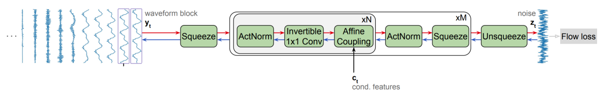
During training (red arrows), the input to the inverse-flow $g^{- 1}$, $y_{t} \in \mathbb{R}^{K}$ is first squeezed into a sequence of $J \in \mathbb{R}^{L}$ frames, each with dimension $L = 10$. Then, the flow is divided into $M$ stages, each operating at a different temporal resolution. This is implemented by interleaving squeeze operations which reshape the sequence between each stage, halving the number of time-steps and doubling the dimension, as illustrated in the following figure. After the final stage, an unsqueeze operation flattens the output $z_{t}$ to a vector in $\mathbb{R}^{K}$. During generation (blue arrows), each operation is inverted and their order is reversed.

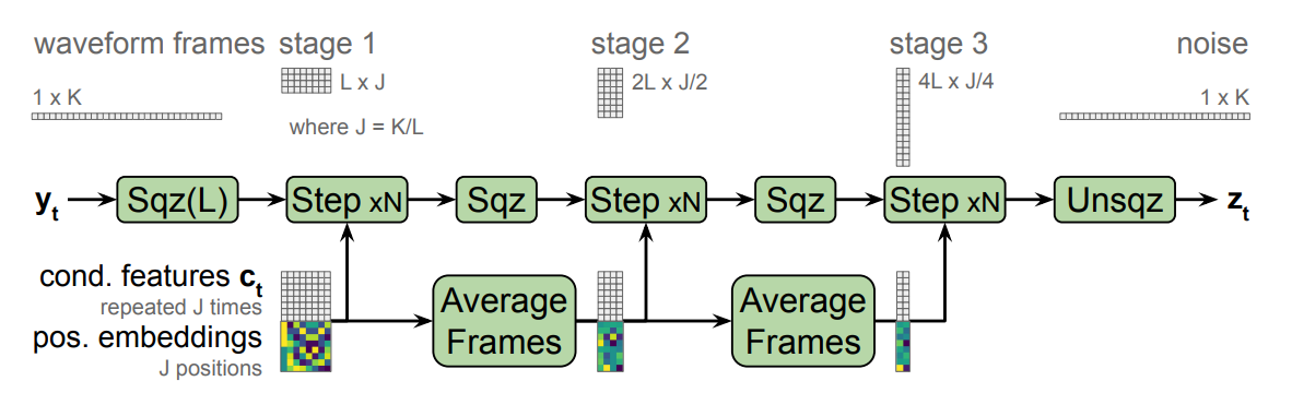
Each stage is further composed of $N$ flow steps. The affine coupling layers emit transformation parameters using a 3-layer 1D convnet with kernel sizes $\lbrack 3,\ 1,\ 3\rbrack$, with $256$ channels. Through the use of squeeze layers, coupling layers in different stages use the same kernel widths yet have different effective receptive fields relative to $y_{t}$. The default configuration uses $M = 5$ and $N = 12$, for a total of 60 steps.

Note:
To understand more about the actNorm, 1x1 convnet, and affine layer used in the normalizing flow network, please review the WaveGlow post where we talked about these components in details.

Loss Function

The overall loss for Wave-Tacotron model is the mean loss of the flow-loss and eos (end-of-sentence) loss all decoder steps $t \in \lbrack 1,T\rbrack$ as shown in the following formula:

The flow loss $\mathcal{L}{flow}$ is the negative likelihood of the flow step to maps the target waveform $y{t}$ to the corresponding $z_{t}$ conditioning on the decoder features $c_{t}$: as shown in the following equation:

The EOS loss $\mathcal{L}_{eos}$,is basically a binary cross entropy loss of predicting that the current step $t$ is the final output step. To obtain the EOS loss, a linear classifier is built on top of $c_t$ to compute the probability ${\widehat{s}}_t$ indicating that $t$ is the final output step knowing the ground truth stop token $s_t$; as shown in the following equation:

Experiments & Results

Experiments in this paper were conducted on LJ Speech dataset which consists of audio book recordings: $22$ hours for training and a held-out $130$ utterance subset for evaluation. They upsampled the recordings to to $24\ kHz$. Also, they used an internal dataset containing about $39$ hours of speech, sampled at $24\ kHz$, from a professional female voice actress. Regarding pre-processing, they used a text normalization pipeline and pronunciation lexicon to map input text into a sequence of phonemes. Wave-Tacotron models were trained using the Adam optimizer for$\ 500k$ steps on 32, with batch size $256$ for the internal dataset and $128$ for LJ, whose average speech duration is longer.

Performance is measured using subjective listening tests, crowd-sourced via a pool of native speakers listening with headphones. Results are measuring using the mean opinion score (MOS) rating naturalness of generated speech on a ten-point scale from 1 to 5. In addition to that, they used several objective metrics such as:

• Mel-Cepstral Distortion (MCD): the root mean squared error against the ground truth signal, computed on $13$ dimensional MFCCs using dynamic time warping to align features computed on the synthesized audio to those computed from the ground truth. MFCC features were computed from an $80$-channel log-mel spectrogram using a $50ms$ Hann window and hop of $12.5ms$. The lower MCD is, the better the performance is.

• Mel-Spectral Distortion (MSD): which is the same as MCD but applied to the log-mel spectrogram magnitude instead of cepstral coefficients. This captures harmonic content which is explicitly removed in MCD due to liftering. The lower MSD is, the better the performance is.

• Character Error Rate (CER): which is computed after transcribing the generated speech with the Google speech API. This is a rough measure of intelligibility, invariant to some types of acoustic distortion. The lower CER is, the better the performance is.

The following table compares between Wave-Tacotron and three other models on LJ speech (first table) and the internal dataset (second table). The first is a Tacotron + WaveRNN model, the second is a Tacotron + Flowcoder model, and the last one is a Tacotron + Post-net (Tacotron-PN), consisting of a 20-layer non-causal WaveNet stack split into two dilation cycles.

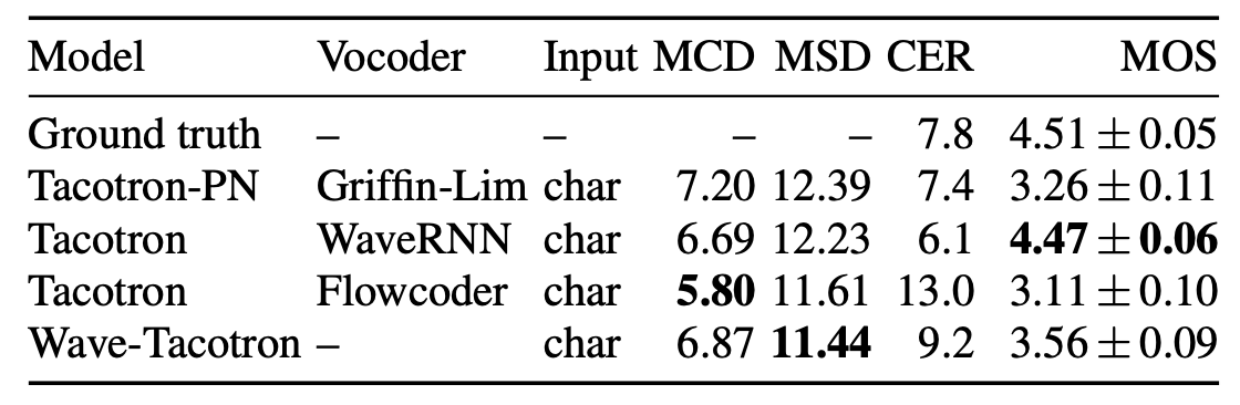
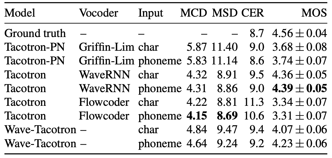
As you can see from the past tables, WaveTacotron is not as well as Tacotron + WaveRNN. Using the flow as a vocoder results in MCD and MSD on par with Tacotron + WaveRNN, but increased CER and low MOS, where raters noted robotic and gravelly sound quality. Wave-Tacotron has higher MCD and MSD than the Tacotron + WaveRNN baseline, but similar CER and only slightly lower MOS. Wave-Tacotron and Flowcoder MSD are lower in LJ speech which is much smaller, leading to the conclusion that fully end-to-end TTS training likely requires more data than the two-step approach.

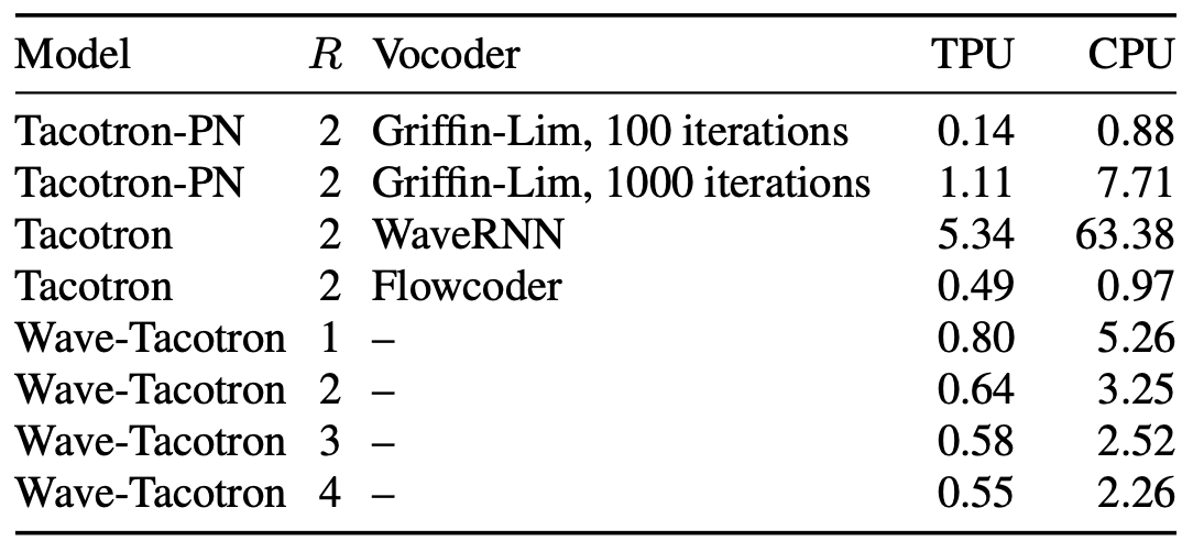
The following table compares the generation speed of audio from input text on TPU and CPU. The baseline Tacotron+WaveRNN has the slowest generation speed, Tacotron-PN is substantially faster, as is Tacotron + Flowcoder. Wave-Tacotron is about $17\%$ slower than Tacotron + Flowcoder on TPU, and about twice as fast as Tacotron-PN using 1000 Griffin-Lim iterations:

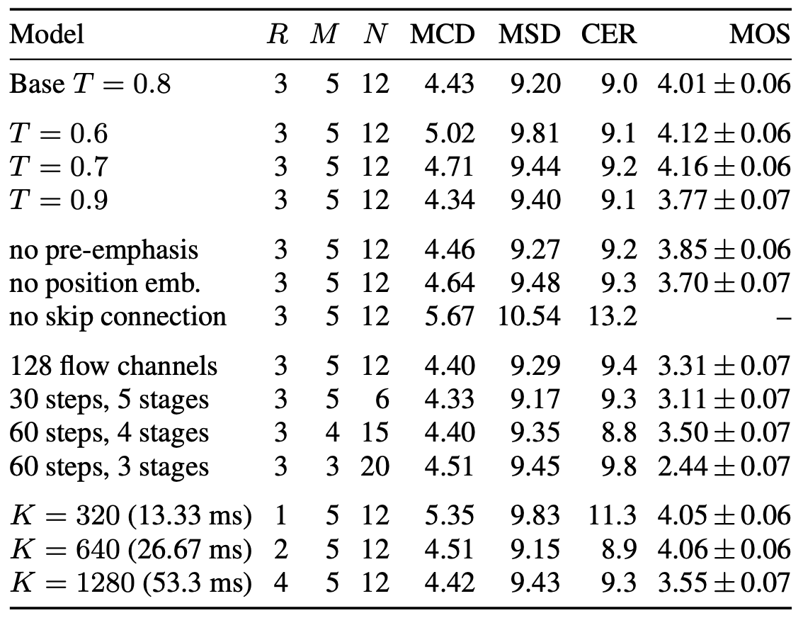
Finally, the following table compares several Wave-Tacotron variations. As shown in the top, the optimal sampling temperature (standard deviation) is $T = 0.7$. Removing pre-emphasis, position embeddings in the conditioning stack, or the decoder skip connection, all hurt performance. Decreasing the size of the flow network by halving the number of coupling layer channels to $128$, or decreasing the number of stages $M$ or steps per stage $N$, all significantly reduce quality in terms of MOS. Finally, reducing $R$ does not hurt MOS, although it slows down generation.