FastSpeech 2
FastSpeech model was a novel non-autoregressive TTS model that achieve on-par results to auto-regressive counterparts while being 38 times faster. Despite these advantages, FastSpeech had three main issues:
-
It was depending on a teacher auto-regressive model making pipeline complicated and time-consuming.
-
The duration extracted from the teacher model was not accurate enough, which hurt the duration predictor performance.
-
The target mel-spectrograms distilled from teacher model suffered from information loss due to data simplification, which limited the voice quality.
FastSpeech 2 is a non-autoregressive TTS model by the same authors as FastSpeech where they solved the issues mentioned above. FastSpeech 2 is trained directly on the ground-truth target instead of the simplified output from the teacher TTS. FastSpeech 2 was proposed by Microsoft (same authors as FastSpeech) in 2020 and published in this paper under the same name: “FastSpeech 2: Fast and High-Quality End-to-End Text to Speech”. The official synthesized speech samples resulted from FastSpeech 2 can be found in this website. The unofficial PyTorch implementation of FastSpeech 2 can be found in this GitHub repository: FastSpeech2.

Architecture
The overall architecture of FastSpeech 2 is shown in the following figure. The Encoder converts the phoneme embedding sequence into the phoneme hidden sequence, and then the Variance Adaptor adds in different variance information such as duration, pitch and energy into the hidden sequence, finally the Mel-spectrogram Decoder converts the adapted hidden sequence into mel-spectrogram sequence in parallel.
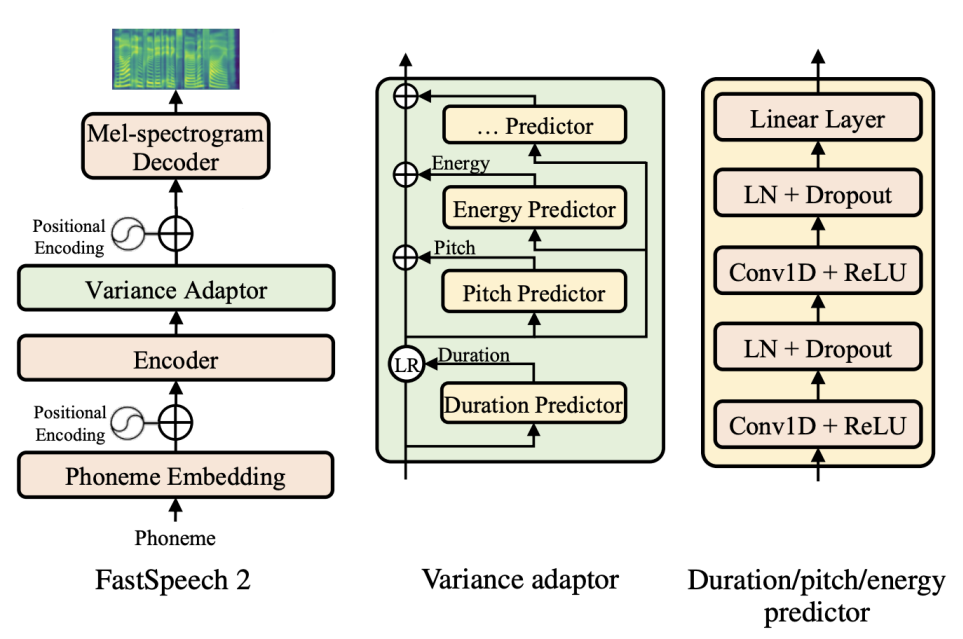
From the previous figure, we can see that FastSpeech 2 consists of three main components: Encoder, Variance Adaptor, and Mel-spectrogram Decoder. In the next part, we are going to discuss each component in more details:
Encoder
The encoder here is the same as the Feed-forward Transformer in FastSpeech which is a stack of $N$ blocks of FFT blocks. Each FFT block, as shown below, consists of multi-head self-attention mechanism to extract the cross-position information and 2-layer 1D convolutional network with ReLU activation. Similar to Transformer, residual connections, layer normalization, and dropout are added after the self-attention network and 1D convolutional network respectively.

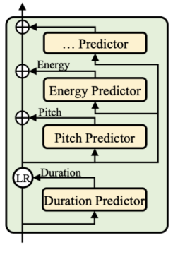
Variance Adaptor
The Variance Adaptor (shown in the following figure) aims to add variance information (e.g., duration, pitch, energy, emotion, style, speaker, … etc.) to the phoneme hidden sequence, which can provide enough information to predict variant speech. As you can see from the figure, they only care for the phone duration, pitch and energy information in the paper. However, the model is flexible and can adapt to more variance information.

On the other hand, the following figure shows the architecture of the duration/pitch/energy predictors. They all share the model structure (but different model parameters), which consists of a 2-layer 1D-convolutional network with ReLU activation, each followed by the layer normalization and the dropout layer, and an extra linear layer to project the hidden states into the output sequence. In the following paragraphs, we describe the details of the three predictors respectively.
Duration Predictor
The Duration Predictor (same as in FastSpeech) takes the phoneme hidden sequence as input and predicts the duration of each phoneme (how many mel frames correspond to this phoneme), and is converted into logarithmic domain for ease of prediction.
It is optimized with mean square error (MSE) loss, taking the extracted duration as training target. Instead of extracting the phoneme duration using a pre-trained autoregressive TTS model in FastSpeech, it uses Montreal forced alignment tool.
Pitch Predictor
“Pitch” is a key feature to convey emotions and greatly affects the speech prosody. To better predict the variations in pitch contour, they used continuous wavelet transform (CWT) to decompose the continuous pitch series into pitch spectrogram and take the pitch spectrogram as the training target for the pitch predictor.
In inference, the pitch Predictor predicts the pitch spectrogram, which is further converted back into pitch contour using inverse continuous wavelet transform (iCWT). To take the pitch contour as input in both training and inference, they quantized pitch $F0$ (ground-truth/predicted value for train/inference respectively) of each frame to $256$ possible values in log-scale and further convert it into pitch embedding vector $p$ and add it to the expanded hidden sequence. Pitch Predictor is optimized with MSE loss.
Energy Predictor
“Energy” indicates the frame-level magnitude of mel-spectrograms and directly affects the volume and prosody of speech. It’s computed as the L2-norm of the amplitude of each short-time Fourier transform (STFT) frame. Then, they quantized the energy of each frame to $256$ possible values uniformly, encoded it into energy embedding $e$ and add it to the expanded hidden sequence similarly to pitch. They used the Energy Predictor to predict the original values of energy instead of the quantized values and optimize the energy predictor with MSE loss.
Mel-spectrogram Decoder
The decoder here is the same as the Feed-forward Transformer in FastSpeech which is a stack of $N$ blocks of FFT blocks. Each FFT block, as shown below, consists of multi-head self-attention mechanism to extract the cross-position information and 2-layer 1D convolutional network with ReLU activation. Similar to Transformer, residual connections, layer normalization, and dropout are added after the self-attention network and 1D convolutional network respectively. The output linear layer in the decoder converts the hidden states into 80-dimensional mel-spectrograms and our model is optimized with mean absolute error (MAE).
FastSpeech 2s
In the paper, they introduced a new variant of FastSpeech2 which doesn’t have the need for Vocoder as it directly generates waveform from text. As shown in the following figure, FastSpeech 2s replaces the mel-spectrogram decoder in FastSpeech 2 with a waveform decoder.
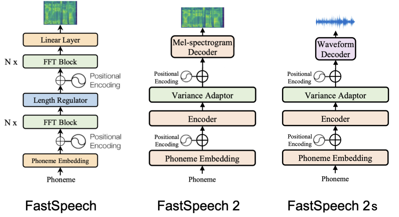
The waveform decoder used in FastSpeech 2, as shown below, has the same architecture as WaveNet including non-causal convolutions and gated activation. The waveform decoder takes a sliced hidden sequence corresponding to a short audio clip as input and up-samples it with transposed 1D-convolution to match the length of audio clip. The waveform decoder consists of 1-layer transposed 1D-convolution with filter size $64$ and $30$ dilated residual convolution blocks, whose skip channel size and kernel size of 1D-convolution are set to $64$ and $3$.

Pushing TTS pipeline towards fully end-to-end framework has several challenges. In this part, we are going to discuss the problem as how the authors tried to overcome it:
-
Challenge: Since the waveform contains more variance information (e.g., phase) than mel-spectrograms, the information gap between the input and output is larger than that in text-to-spectrogram generation.
- Solution: They used adversarial training to force the decoder to implicitly recover the phase information by itself. The discriminator in the adversarial training adopts the same structure in Parallel WaveGAN which consists of ten layers of non-causal dilated 1-D convolutions with leaky ReLU activation function.
-
Challenge: It is difficult to train on the audio clip that corresponds to the full text sequence due to the extremely long waveform samples and limited GPU memory.
- Solution: They leveraged the mel-spectrogram decoder of FastSpeech 2, which is trained on the full text sequence to help on the text feature extraction.
The waveform decoder is optimized by the multi-resolution STFT loss and the LSGAN discriminator loss following Parallel WaveGAN. In inference, they discarded the mel-spectrogram decoder and only use the waveform decoder to synthesize speech audio.
Experiments
Similar to FastSpeech, all experiments in this paper was done on LJSpeech dataset which contains $13,100$ English audio clips (about 24 hours) and corresponding text transcripts. Unlike FastSpeech, they split the dataset differently: they used $12,228$ samples for training, $349$ samples (with document title LJ003) for validation and $523$ samples (with document title LJ001 and LJ002) for testing. For subjective evaluation, they randomly choose 100 samples in test set.
Similarly to FastSpeech, as a pre-processing step, they converted the text sequence into the phoneme sequence using grapheme-to-phoneme (g2p) tool. And they converted the raw waveform into mel-spectrograms using frame size of $1024$ and hop size of $256$ with respect to the sample rate $22050$.
Regarding the model configuration, FastSpeech 2 consists of 4 feed-forward Transformer (FFT) blocks in the encoder and the mel-spectrogram decoder. The output linear layer in the decoder converts the hidden states into 80-dimensional mel-spectrograms and the model is optimized with mean absolute error (MAE).
To train FastSpeech 2, they used the Adam optimizer with $\beta_{1} = 0.9$, $\beta_{2} = 0.98$, and $\epsilon = 10^{- 9}$. FastSpeech 2 takes double the number of training steps for training until convergence than FastSpeech, it takes $160k$ steps. In the inference process, they used a pre-trained Parallel WaveGAN as a Vocoder. The total list of hyper-parameters used in this model can be seen below:
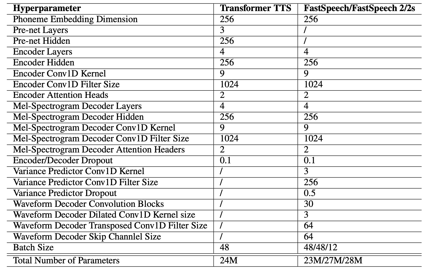
For FastSpeech 2s, they used the same optimizer and learning rate schedule as FastSpeech 2, and it took the model $600k$ steps for training until convergence. The details of the adversarial training follow Parallel WaveGAN.
Results
In this part, we are going to discuss the performance of FastSpeech 2 in terms of:
- Audio Quality:
They compared FastSpeech 2 to the ground-truth with/without Vocoder, Tacotron 2, Transformer TTS, and FastSpeech. All previous models used Parallel WaveGAN (PWG) as vocoder. The results are shown in the following table which shows that FastSpeech 2 outperforms FastSpeech and other auto-regressive models. can nearly match the quality of the Transformer TTS and Tacotron 2 models.

- Inference Speedup:
They compared the inference of FastSpeech 2 compared to Transformer TTS model and FastSpeech and results are shown in the following table. FastSpeech 2 simplifies the training pipeline of FastSpeech by removing the teacher-student distillation process, and thus reduces the training time by $3.12$x compared with FastSpeech.
