data2vec
data2vec is a framework proposed by Meta in 2022 that uses self-supervised learning on “speech, text, and image” modalities to create a single framework that works for all three. So, instead of using word2vec, wav2vec, or image2vec, we can use data2vec instead. This work could be a step closer to models that understand the world better through multiple modalities. data2vec was published in this paper: data2vec: A General Framework for Self-supervised Learning in Speech, Vision and Language. The official code for data2vec can be found as part of Fairseq framework on GitHub: fairseq/data2vec.
The core idea behind data2vec is instead of predicting modality-specific targets (e.g speech-units, sub-words, or visual tokens), data2vec is trained to predict contextualized latent representations (layers’ weights) which removes the dependence on modality-specific targets in the learning task. In the next part, we are going to see how data2vec made this possible.
Feature Encoding
Given an input data of different modalities (images, audio, and text), data2vec first uses modality-specific encoders to encode these inputs. The following are the different encoders used per modality:
- Computer Vision:
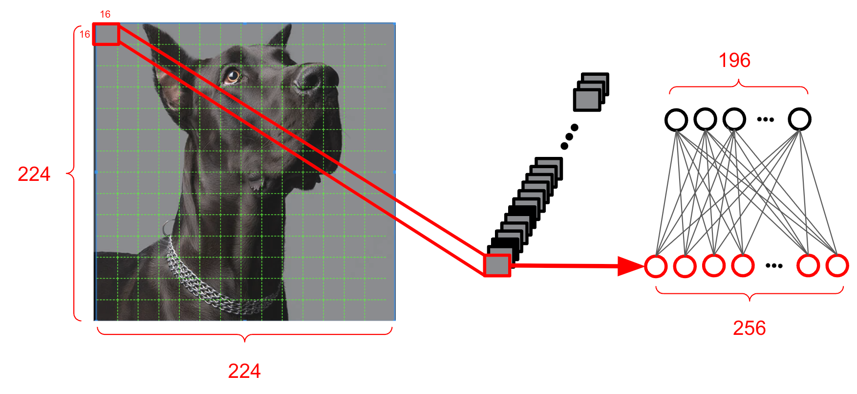
They used the ViT (Vision Transformer) strategy of taking $224 \times 224$ images as input and treats them as a sequence of fourteen $16 \times 16$ patches. Then, each patch is linearly transformed and a sequence of $196$ representations.
- Speech Processing:
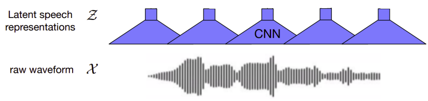
They used the “feature encoder” module of the Wav2Vec 2.0 model which consists of $7$ temporal convolutions with $512$ channels, strides $\lbrack 5,2,2,2,2,2,2\rbrack$ and kernel widths $\lbrack 10,3,3,3,3,2,2\rbrack$. This results in an encoder output frequency of $50\ Hz$ with a stride of about $20ms$ between each sample, and a receptive field of $400$ input samples or $25ms$ of audio. The raw waveform input to the encoder is normalized $(\mu = 0,\ \sigma = 1)$.
- NLP:
They used the word embeddings layer of RoBERTa, which is Meta’s re-implementation of BERT after tokenized the input textual data using a byte-pair encoding (BPE) of $50K$ tokens.
Pre-Training
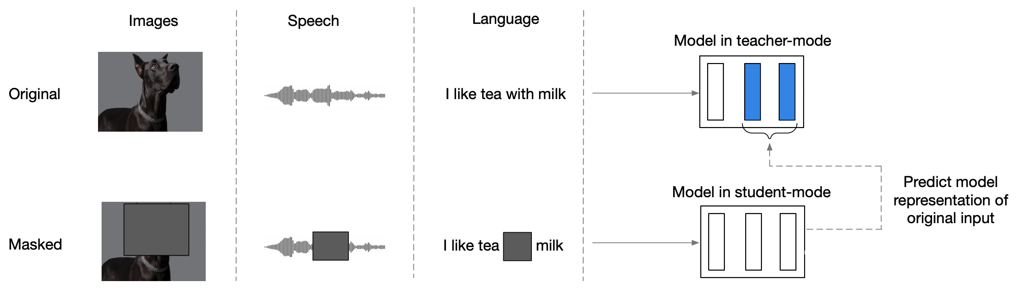
Now that all three different modalities have been encoded into encodings, the next step is to train data2vec model using these encodings as input; which is done in two modes simultaneously (at the same time) as shown in the following figure:
-
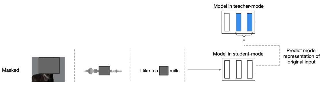
Teacher Mode:
data2vec model uses the input encodings (without masking) to produce latent representations. -
Student Mode:
The same data2vec model uses masked encodings, produced using different masking strategy depending on the modality, and tries to restore the same latent representations formed in the top-K layers of the teacher mode.
Notes:
In this paper, they used the standard Transformer-encoder architecture as the data2vec model. However alternative architectures may be equally applicable.
Teacher Mode
In this part, we are going to discuss the data2vec training in the teacher mode. In this mode as shown in the following figure, the data2vec model is trained from scratch using unmasked encodings to predict these input encodings.

In this mode, the data2vec model works as an AutoEncoder. However, the encodings in data2vec are parameterized by Exponentially Moving Average (EMA) according to the following equation:
\[\theta_{t} \leftarrow \tau\theta_{t} + (1 - \tau)\theta_{s}\]Where $\theta_{t}$ and $\theta_{s}$ are the model weights in the teacher-mode and student-mode respectively, $\tau$ is a scheduler that linearly increases over time from a starting value $\tau_{0}$ to a final value $\tau_{e}$ over $\tau_{n}$ updates. After which, the value is kept the same for the remainder of training. This leads to the teacher being updated more frequently at the beginning of training, when the model is random, and less frequently later in training, when good parameters have already been learned.
During training in teacher mode, data2vec constructs training targets for the student mode. More formally, given a data2vec network $f_{t}$ of $L$ total layers, the layer’s output at time-step $t$ (denoted as $a_{t}^{l}$) is the last residual connection. The training targets are constructed using the top $K$ layers according to the following steps:
-
For every layer $l$, the top $K$ layers are nomralized at every time-step $t$ to obtain ${\widehat{a}}_{t}^{l}$.
-
Then, all outputs of the top $K$ layers are averaged together:
\[y_{t} = \frac{1}{K}\sum_{l = L - K + 1}^{L}{\widehat{a}}_{t}^{l}\] -
Finally, given an input $x$ and training targets $y_{t}$, a smooth L1 loss is used to train data2vec in student mode where $\beta$ controls the transition from a squared loss to an L1 loss, depending on the size of the gap between the teacher’s prediction $y_{t}$ and the student prediction $f_{t}(x)$ at time-step $t$. The advantage of this loss is that it is less sensitive to outliers:
Notes:
For speech representations, they used instance normalization without any learned parameters, while for NLP and vision they used parameter-less layer normalization.
The targets resulted from the teacher mode are “contextualized targets” since it incorporates information about the entire input instead of part of the input as it happens with wav2vec.
Student Mode
Now that we are familiar with how training happens in the teacher mode along with how the training targets are created. Let’s see how data2vec model is trained in the student mode.
As shown in the previous figure, the first thing that happens is masking the input encodings which differs based on the input data modality. The following are the different masking strategies used in the student mode depending on the input modality:
-
Computer Vision:
They followed the BEiT paper by masking blocks of multiple adjacent patches. Different to the previous work, they found it’s better to mask $60\%$ of the patches instead of $40\%$. -
Speech Processing:
The masking strategy is also identical to Wav2Vec 2.0 as they sample $p = 0.065$ of all time-steps to be starting indices and mask the subsequent $10$ time-steps. This results in approximately $49\%$ of all time-steps to be masked for a typical training sequence. -
NLP:
They used BERT masking strategy to mask $15\%$ of uniformly selected tokens; such as that $80\%$ are replaced by a learned mask token, $10\%$ are left unchanged and $10\%$ are replaced by randomly selected vocabulary token. They also explored using wav2vec 2.0 strategy of masking spans of four tokens.
After masking the data encodings, the model is trained to predict the training targets constructed in the teacher mode.
Note:
After pretraining, they use data2vec as the encoder and fine-tune it on labeled data and train it to minimize a cross-entropy (CE) criterion.
Experiments & Results
The main architecture for data2vec is the Transformer architecture. In the paper, they created two different sizes of data2vec: data2vec Base and data2vec Large, containing parameters as shown in the following table; and they trained data2vec on a modality-specific task as we are going to see next.
| $$L$$ | $$d_{m}$$ | $$d_{\text{ff}}$$ | $$h$$ | |
|---|---|---|---|---|
| Base | 12 | 768 | 3072 | 12 |
| Large | 6 | 1024 | 4096 | 16 |
Computer Vision
They pre-trained the two sizes of data2vec on images from ImageNet-1K training set according to the hyper-parameters shown in the following table; for optimization, they used Adam optimizer with consine schedule with a single cycle where they warm up the learning rate. Also, they use a constant value $\tau$ of with no schedule.
| $$\beta$$ | $$bs$$ | $$K$$ | $$\tau$$ | $${lr}_{start}$$ | $${lr}_{end}$$ | warmup epochs | train epochs | |
|---|---|---|---|---|---|---|---|---|
| Base | 2 | 2048 | 6 | 0.9998 | 0.002 | 0.001 | 40 | 800 |
| Large | 2 | 8192 | 6 | 0.9998 | 0.002 | 0.001 | 80 | 1600 |
After pre-training, they fine-tuned the resulting model for image classification task using the labeled data of the same benchmark. To do so, they average-pooled the output of the last layer and input it to a softmax-normalized classifier. Fine-tuning was done according to the following hyper-parameters:
| $$lr$$ | warmup epochs | finetuning epochs | |
|---|---|---|---|
| Base | 0.004 | 20 | 100 |
| Large | 0.004 | 5 | 50 |
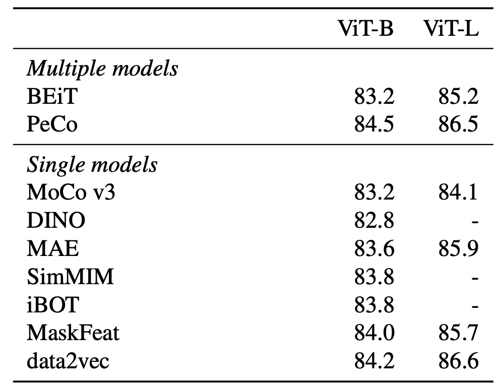
Following standard practice, models were evaluated in terms of top-1 accuracy on the validation set. The following table shows that data2vec outperforms prior work with both base and large sizes in the single model; and large size in the multiple models.
Speech Processing
They pre-trained the two sizes of data2vec on the 960 hours LibriSpeech, which contains speech from audiobooks in English, according to the hyper-parameters shown in the following table:
| $$bs$$ | $$K$$ | $$\tau_0$$ | $$\tau_e$$ | $$\tau_n$$ | train updates | |
|---|---|---|---|---|---|---|
| Base / Large | 63 mins | 8 | 0.999 | 0.9999 | 30k | 400k |
For optimization, they used Adam optimizer with a peak learning rate of $5 \times 10^{- 4}$ with a tri-stage scheduler which linearly warms up the learning rate over the first $3\%$ of updates and holds it for $90\%$ and then linearly decays it over the remaining $7\%$. The following table shows the results on librispeech test-other when fine-tuning pre-trained models on the libri-light low-resource labeled data. As you can see, improvements can be seen when adding more and more labeled data across both data2vec sizes surpassing other models such as wav2vec 2.0, HuBERT, and WavLM.

To further validate these results, they also used the AudioSet benchmark where they used the same pre-training hyper-parameters as before while increasing $K$ to $12$ and training for fewer steps ($200k$) with bigger batch size ($94.5\ mins$). Also, they applied DeepNorm and layer normalization to stabilize pre-training. Finetuning was done on the balanced subset for $13k$ steps and a batch size of $21.3\ mins$. Results are shown in the following table which shows that data2vec can outperform comparable setups that uses the same pre-training and fine-tuning data:

NLP
They pre-trained data2vec on the same pretraining setup of BERT on the Books Corpus and English Wikipedia data using Adam optimizer with a tri-stage learning scheduler according to the following hyper-parameters:
| $$bs$$ | $$K$$ | $$\beta$$ | $$\tau_0$$ | $$\tau_e$$ | $$\tau_n$$ | train updates | |
|---|---|---|---|---|---|---|---|
| Base | 256 | 10 | 4 | 0.999 | 0.9999 | 100k | 1M |
After pre-training, they fine-tuned the result model on the GLUE benchmarks separately on the labeled data provided by each task. The average accuracy on the development sets over fine fine-tuning runs are reported below:

The previous table shows that data2vec outperforms RoBERTa baseline and its performance is improved once using the wav2vec 2.0 masking that spans four tokens.
Ablation
To examine the impact of different components about data2vec, authors have performed multiple ablation studies as we are going to see next:
- Top-K layers:
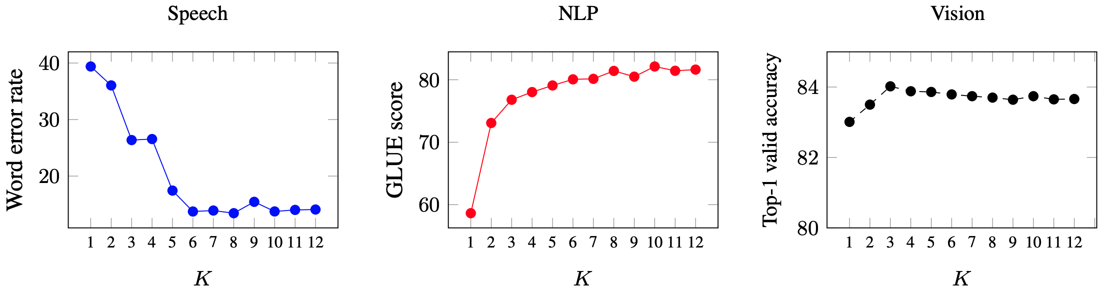
They measured the performance across all three modalities when average the top-K layers of the teacher mode that are used to create the training targets for the student model. For faster training, they used the data2vec base model. Results are shown in the following figure where we can see that “speech” needs more averaging deeper layers unlike “NLP” and “Vision”.
- Masked Ratio:
They measures the effect of masked ratio on the performance. So, they masked all but a fraction of the data when constructing the target representations in the teacher for pre-training and report downstream performance for speech and vision.
