BEST-RQ
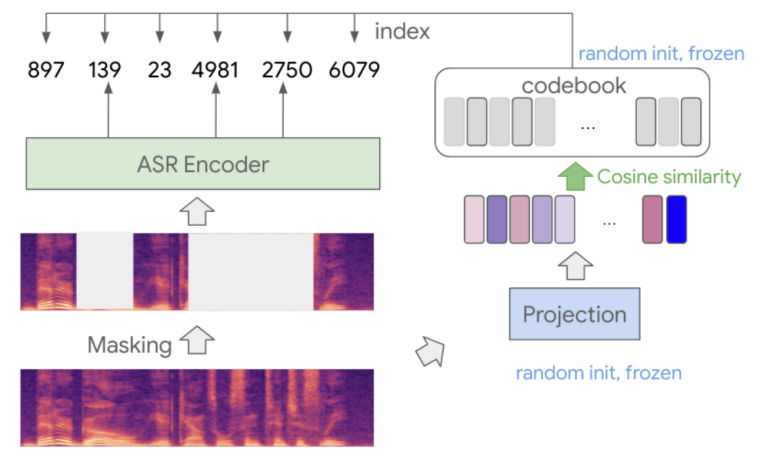
BEST-RQ stands for “BERT-based Speech pre-Training with Random-projection Quantizer” which is a BERT-like self-supervised learning technique for speech recognition. BEST-RQ masks input speech signals and feeds them to an encoder which learns to predict the masked labels using the unmasked labels. Both masked and unmaksed labels are provided by a random-projection quantizer as shown in the following figure. BEST-RQ was proposed by Google Brain in 2022 and published in this paper: Self-Supervised Learning with Random-Projection Quantizer for Speech Recognition.
As you might have noticed, this work seems very similar to other BERT-like self-supervised training approaches such as:
-
vq-wav2vec which quantizes the continuous representation of wav2vec to discrete tokens and performs BERT-like masking during pre-training.
-
wav2vec 2.0 which quantizes the input speech using vq-wav2vec and then combines contrastive learning with BERT-like masking where the model has to identify the quanitzed representation among different distractors.
-
HuBERT which quantizes the input speech using k-means and then performs BERT-like masking to pre-train the initial version. Then, the pre-trained HuBERT is used as a quantizer for following epochs.
-
w2v-BERT uses quantizes the input speech using wav2vec 2.0 and then use BERT-like masking during pre-training.
Pre-training
BEST-RQ pre-training, as shown in the previous figure, can be divided into the following steps steps:
-
The input speech is normalized to have mean $\mu = 0$ and standard deviation $\sigma = 1$. This normalization step is critical for preventing the quantizer to collapse to a small subset of codes.
-
BEST-RQ masks the input speech signal differently than earlier techniques. It applies masking at every frame with a fixed probability $p$, and with a fixed span length. The masked parts are then replaced with a noise sampled from a normal distribution $\mathcal{N}(0,\ 0.1)$.
-
Then, the masked and unmasked segments are quantized using random-projection quantizer. More formally, given an input speech vector $x \in \mathbb{R}^{d}$, the random-projection quantizer maps $x$ to discrete labels $y$ through the following formula where $x \in \mathbb{R}^{h \times d}$ denotes a randomly initialized matrix using Xavier initialization, and $C = \left\{ c_{1},\ …c_{n} \right\}$ is a set of randomly initialized $h$-dimenstional vectors from a normal distribution. The quantizer uses the matrix $A$ to project the input speech signals and the codebook $C$ and cosine similarity is used to find the nearest vector where the index of the vector is the label.
- Finally, the quantized segments are fed to the ASR encoder. A softmax layer is added on top of the encoder and the encoder is trained to predict the labels of the masked part. In the paper, they used the Conformer-based encoder.
Note:
Both the randomly initialized matrix $A$ and codebook $C$ are fixed during the pre-training process.
Experiments & Results
In this section, we are going to discuss the different experiments they have performed in the paper and observe the results across different tasks.
Speech Recognition
For pre-training, they used LibriLight dataset, the mask length was $400ms$ with masking probability of $p = 0.01$. The input speech signals are $80$-dimensional log-mel filter bank coefficients, and each frame has the stride of $10ms$. The encoder used consisted of two convolution layers before the 24-layer Conformer forming $0.6B$ parameters. For pre-training, they used Adam optimizer with $0.004$ peak learning rate and $25000$ warmup steps and $2048$ batch size. Since the encoder has $4$ times temporal-dimension reduction due to the two convolution layers, the quantization with random projections stacks every $4$ frames for projections. The vocab size of the codebook is $8192$ and the dimension is $h = 16$.
For fine-tuning, they used LibriSpeech. Regarding the model, they used RNN-Transducer architecture with the pre-trained encoder and the decoder is a two-layers unidirectional LSTM network with a hidden dimention of $1280$ and $1024$-token WordPiece vocabulary. The fine-tuning process use a lower learning rate for the encoder than the decoder. The encoder uses $0.0003$ peak learning rate and $5000$ warmup steps, while the decoder uses $0.001$ peak learning rate and $1500$ warmup steps. The LM is an 8-layers Transformer model with $4096$ feed-forward dimension and $1024$ model dimension, trained on the LibriSpeech text corpus.
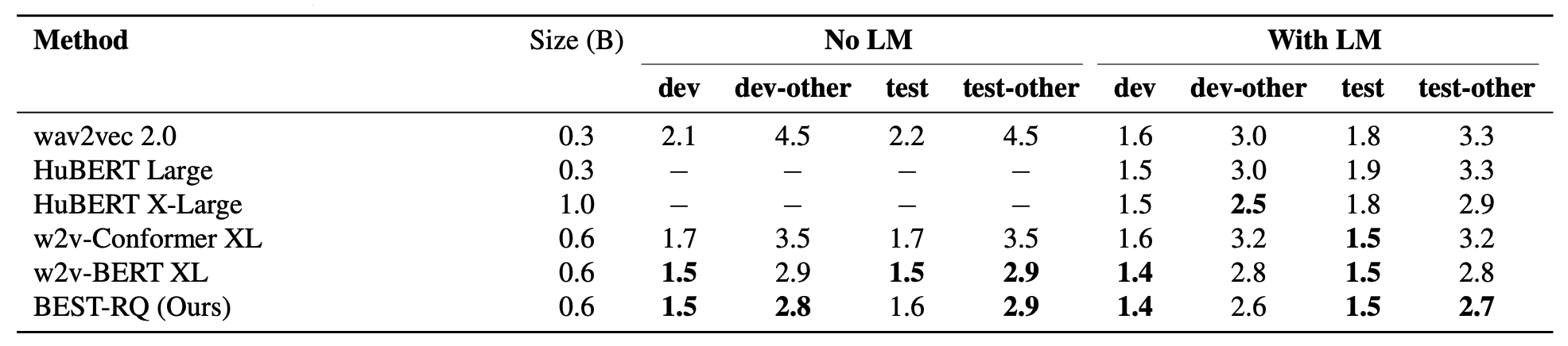
Results, shown in the following table, indicate that BEST-RQ achieves the best results across different dev and test sets in comparison with wav2vec 2.0, HuBERT and w2v-BERT with or without the usage of language model.
Streaming Speech Recognition
To adapt BEST-RQ for streaming speech recognition, they changed the number of layers a little bit while maintaining the same number of parameters ($0.6B$). They used 3 convolutional layers at the bottom (instead of two in non-streaming setup), followed by a stack of $20$ Conformer layer with $1024$ hidden dimension for the self-attention layer and $4096$ for the feed-forward layers. The self-attention layer attends to the current and the previous $64$ frames, and the convolution has a kernel that covers the current and the past $3$ frames.
For pre-training, they tried two different setups:
-
The streaming pre-training: decreases the mask length to $300ms$ instead of $500ms$ and increases the masking probability to $p = 0.02$ instead of $0.01$. The random-projection quantizer stacks every $2$ frames for projections instead of $4$.
-
The non-streaming pre-training: extends the convolution kernel within the Conformer layer to have access for the future $3$ frames. However, the self-attention is still limited to having access only for the previous context. The masking length is kept at $400ms$ and the masking probability is increased to $p = 0.02$.
For fine-tuning, they used RNN-T architecture and 1-layer decoder of unidirectional LSTM with $640$ hidden dimension. The training setup is the same as the fine-tuning config for the non-streaming experiments. When initializing from a non-streaming pre-trained model, the convolution only uses the kernel weight that accesses the previous context to keep the model streaming.
Results on streaming LibriSpeech speech recognition is shown in the following table. These results show that BEST-RQ outperforms wav2vec2.0 and w2v-BERT same masking and training setup as BEST-RQ on both WERs and latency.
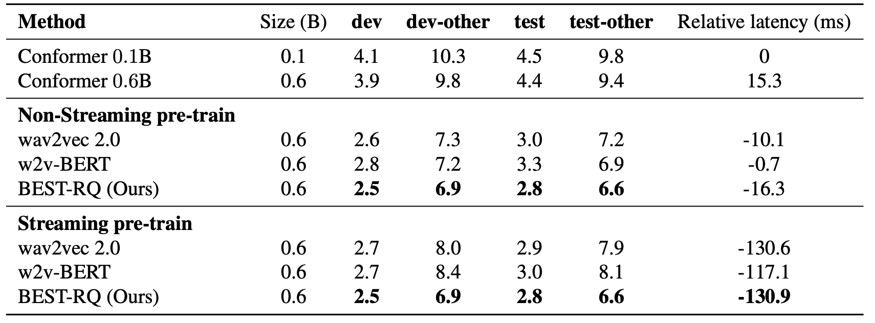
The relative latency, seen in the previous table, is calculated by averaging the timing difference of all matched words between two models according to the following formula where $i$ denotes the index of the matched words, $j$ is the utterance index, $s_{ij}$ and $e_{ij}$ correspond to the starting and ending time of the word from the baseline model, ${s’}{ij}$ and ${e’}{ij}$ correspond to the starting and ending time of the word from the compared model, and $N$ is the total number of matched word among all utterances.
\[\sum_{i,j}^{}\frac{s'_{ij} - s_{ij} + e'_{ij} - e_{ij}}{2N}\]Note:
A negative relative latency means the compared model has lower latency than the baseline model.
Multilingual Speech Recognition
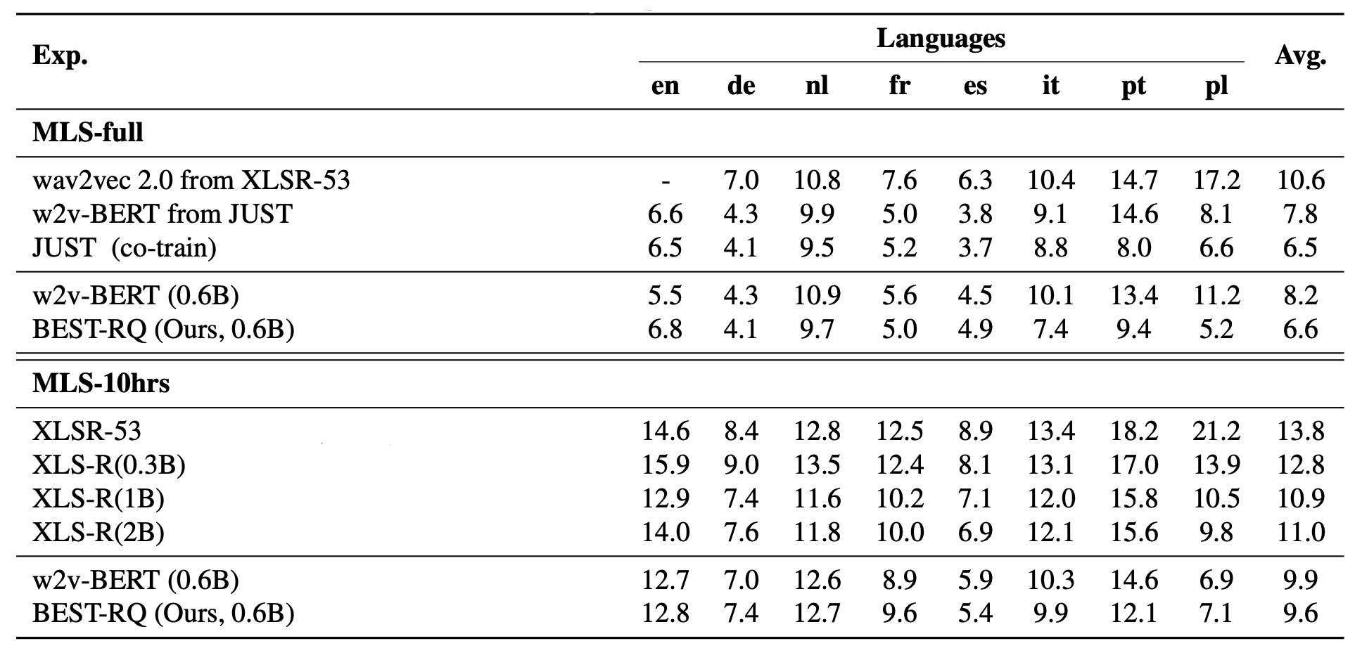
For pre-training, they couldn’t use VoxLingua-107 dataset due to license constraint. So, they created their own version of approximately $429k$ hours of unlabeled speech data in $51$ languages which is $6.6k$ hours smaller than the dataset used to train XLS-R that were trained on $128$ languages. For multilingual ASR fine-tuning, they used MLS dataset containing $50k$ hours spanning 8 languages. For few-shot learning, they used the official $10$ hours split.
As shown in the following table, their w2v-BERT baseline already outperforms previous strong model XLS-R ($2B$). The average WER further bring down by $3\%$ relative by using BEST-RQ. This demonstrate a simple random-projection quantizer is also effective for multilingual pre-training. Interestingly, with more fine-tune data, BEST-RQ perform even better than w2v-BERT, especially for “pt” and “pl” and on-par with XLS-R.
Multilingual Voice Search
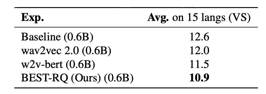
For pre-training, they collected a multilingual Youtube dataset spanning 12 languages and fine-tuned it on VS-1000hrs. Results show that BEST-RQ consistently outperform w2v-BERT and wav2vec 2.0 by $9\%$ and $5\%$ respectively. Compare to w2v-BERT, our proposed method outperform on all the languages.
Analzing the Quantizer
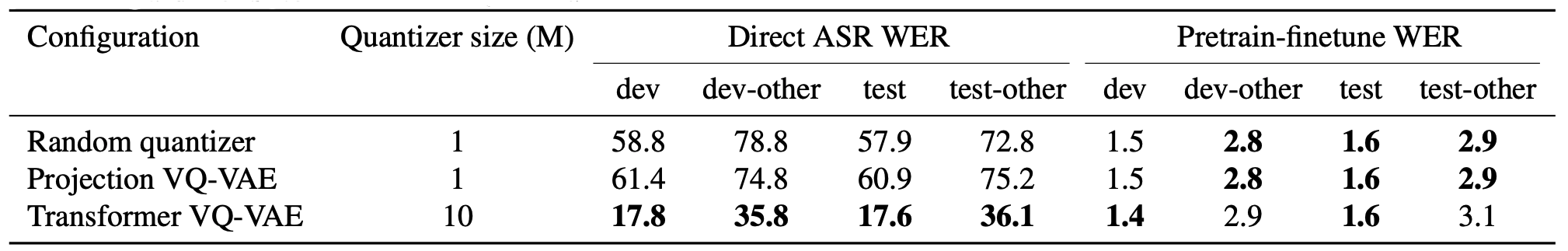
To analyze the effect of the quantizer, they created a smaller version of BEST-RQ with only $25M$ total parameters. This version consists of $16$ Conformer layer with $256$ dimension, $8$ attention heads, $128$ context length and kernel size $5$ for lightweight convolution. Then, they tried three different quantizers:
-
Random-projection quantizer
-
VQ-VAE with projection quantizer
-
Transformer VQ-VAE quantizer.
Results show that even though the Transformer-based quantizer gets much better performance when used as input directly, the random-projection quantizer is equally effective for self-supervised learning.
One potential explanation for the above observation, that a sub-optimal quantization can work well for self-supervised learning, is that the self-supervised learning algorithm can learn to mitigate the quality gap given sufficient amounts of pre-training data.
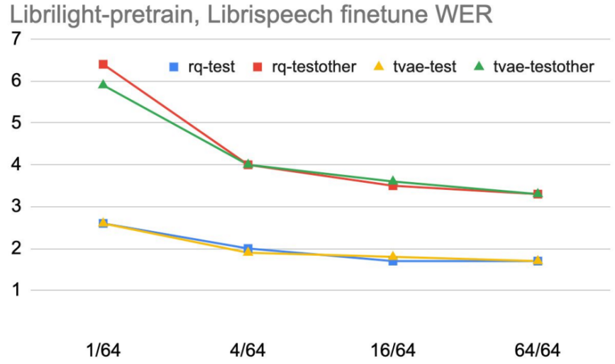
They investigated whether a quantizer with a better quantization quality performs better when the amount of the pre-training data is limited. They compared un-trained random-projection quantizer (rq) and a trained transformer-based VQ-VAE quantizer (tvae) with different pre-training data sizes: $\left\{ 1/64,\ 4/64,\ 16/64,\ 64/64 \right\}$ of LibriLight data for $100k$ steps and a batch size of $2048$. Then, the pre-trained models are fine-tune on LibriSpeech $960h$. The results in the following figure show that a quantizer with better representation quality (Transformer-based VQ-VAE) performs better when pre-training data is limited, but the gap disappears as the pre-training data increase.