VITS

VITS stands for “Variational Inference with adversarial learning for Text-to-Speech”, which is a single-stage non-autoregressive Text-to-Speech model that is able to generate more natural sounding audio than the current two-stage models such as Tacotron 2, Transformer TTS, or even Glow-TTS. VITS was proposed by Kakao Enterprise in 2021 and published in this paper: “Conditional Variational Autoencoder with Adversarial Learning for End-to-End Text-to-Speech”. The official implementation for this paper can be found in this GitHub repository: vits. The official synthetic audio samples resulting from VITS can be found in this website.

Note to Reader:
VITS is just a combination of a lot of ideas from other models. In order to make the best use out of this post, I think you should go through the following posts in order: the “Generative Models Recap” part in the WaveGlow post, the WaveNet post, and the HiFi-GAN post.

Architecture

The overall architecture of the VITS is shown in the following figure. As we, can see VITS consists of a Posterior Encoder, Prior Encoder, Decoder, and Stochastic Duration Predictor. The Posterior Encoder and Decoder’s Discriminator modules are only used during training, not for inference. In the next part, we are going to tackle every component in more details:

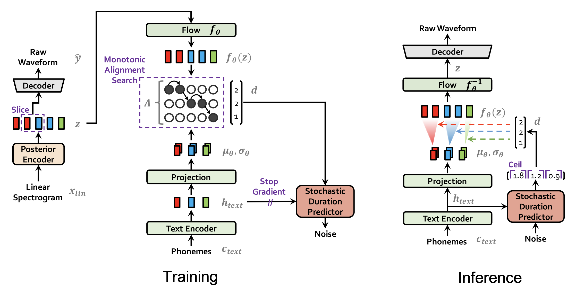
Posterior Encoder

For the posterior encoder, they used 16 WaveNet residual blocks which consists of layers of dilated convolutions with a gated activation unit and skip connection. The posterior encoder takes linear-scale log magnitude spectrograms $x_{lin}$ as input and produces latent variables $z$ with $192$ channels.

The idea behind the Posterior Encoder is to map the audio data from the mel-spectrogram space to a normal-distribution space. That’s why in the paper, they used a linear layer on top of the Posterior Encoder to produce the mean and variance of the normal posterior distribution.

Prior Encoder

The prior encoder consists of different components as you can see from the following figure. It consists of a Text Encoder , a Projection Layer, a Normalizing Flow, and it uses Monotonic Alignment Search (MSA) algorithm. Similar to the Posterior Encoder, the Prior Encoder is aiming at mapping the textual data from the phoneme space to a normal distribution space.

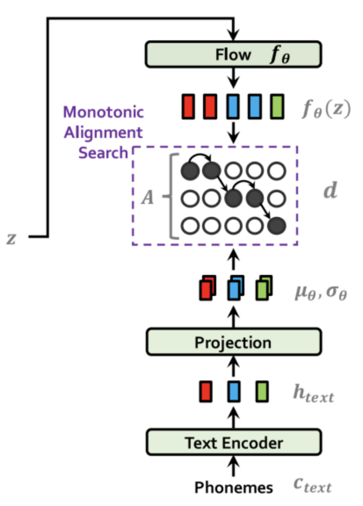
The text encoder is a Transformer- encoder that uses relative positional representation instead of absolute positional encoding (as used in the original paper) which processes the input phonemes $c_{text}$ and results in hidden representations $h_{text}$. Then, a linear projection layer is used to produce the mean $\mu_{\theta}$ and variance $\sigma_{\theta}$ used for constructing the prior distribution.

On the other end, a normalizing flow $f_{\theta}$ is used to improve the flexibility of the prior distribution, which is a stack of four affine coupling layers, each coupling layer consisting of four WaveNet residual blocks as shown in the following figure.

The normalizing flow takes the latent variables $z$ resulting from the Posterior Encoder and outputs latent representation $f_{\theta}(z)$. The MSA algorithm (same as the one used with Glow-TTS) uses the representations from the flow module $f_{\theta}(z)$ and the projection layer $\left( \mu_{\theta},\ \sigma_{\theta} \right)$ to find the optimal alignment $d$.

Note:
The dimension of Flow-based Module output $f_{\theta}(z)$ has the same dimensions as the Posterior Encoder output $z$ with $192$ channels, since either of them can be used as an input to the Decoder depending on the process whether it’s training or inference.

Decoder

The decoder is essentially the HiFi-GAN V1 generator. It is composed of a stack of transposed convolutions, each of which contains multi-receptive field fusion module (MRF) as shown in the following figure.

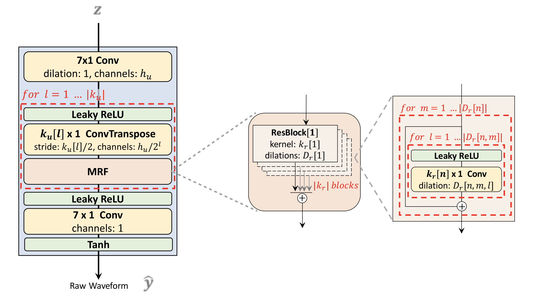
During training, the input of the decoder is latent variables generated from the posterior encoder $z$; while it is the latent variables generated from the prior encoder $f_{\theta}(z)$ during inference. For the last convolutional layer of the decoder, they removed the bias parameter, as it caused unstable gradient scales during mixed precision training.

Regarding the discriminator, they followed the discriminator architecture of the Multi-Period Discriminator (MPD) proposed in HiFi-GAN as shown in the following figure.

For the discriminator, HiFi-GAN uses the multi-period discriminator containing five sub-discriminators with periods $\lbrack 2,\ 3,\ 5,\ 7,\ 11\rbrack$ and the multi-scale discriminator containing three sub-discriminators. To improve training efficiency, they left only the first sub-discriminator of the multi-scale discriminator that operates on raw waveforms and discarded two sub-discriminators operating on average-pooled waveforms. The resultant discriminator can be seen as the multi-period discriminator with periods $\lbrack 1,\ 2,\ 3,\ 5,\ 7,\ 11\rbrack$.

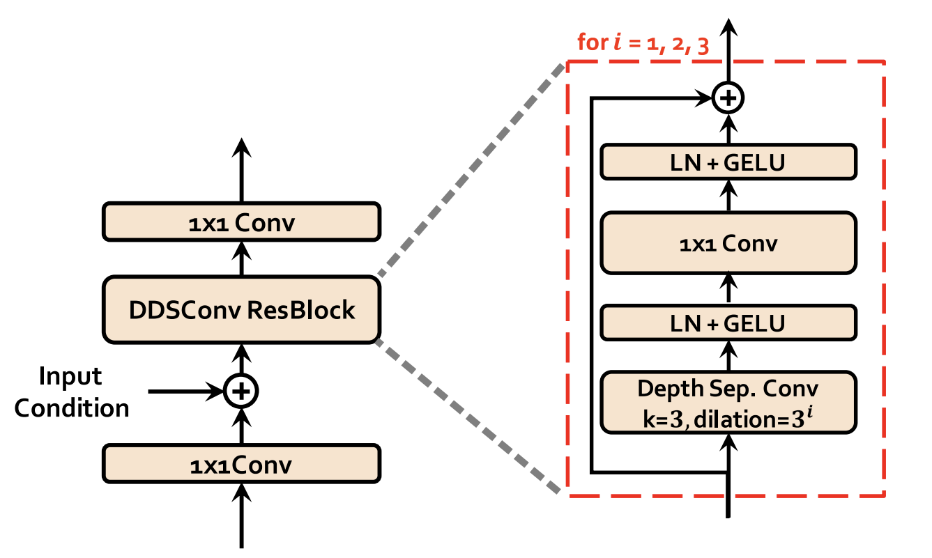
Stochastic Duration Predictor

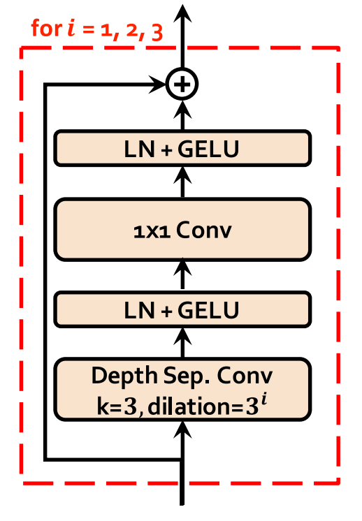
The stochastic duration predictor estimates the distribution of phoneme duration $d$ from a conditional input $h_{text}$ resulting from the Text Encoder + Projection Layer. The following figure shows the training and inference procedures of the stochastic duration predictor.

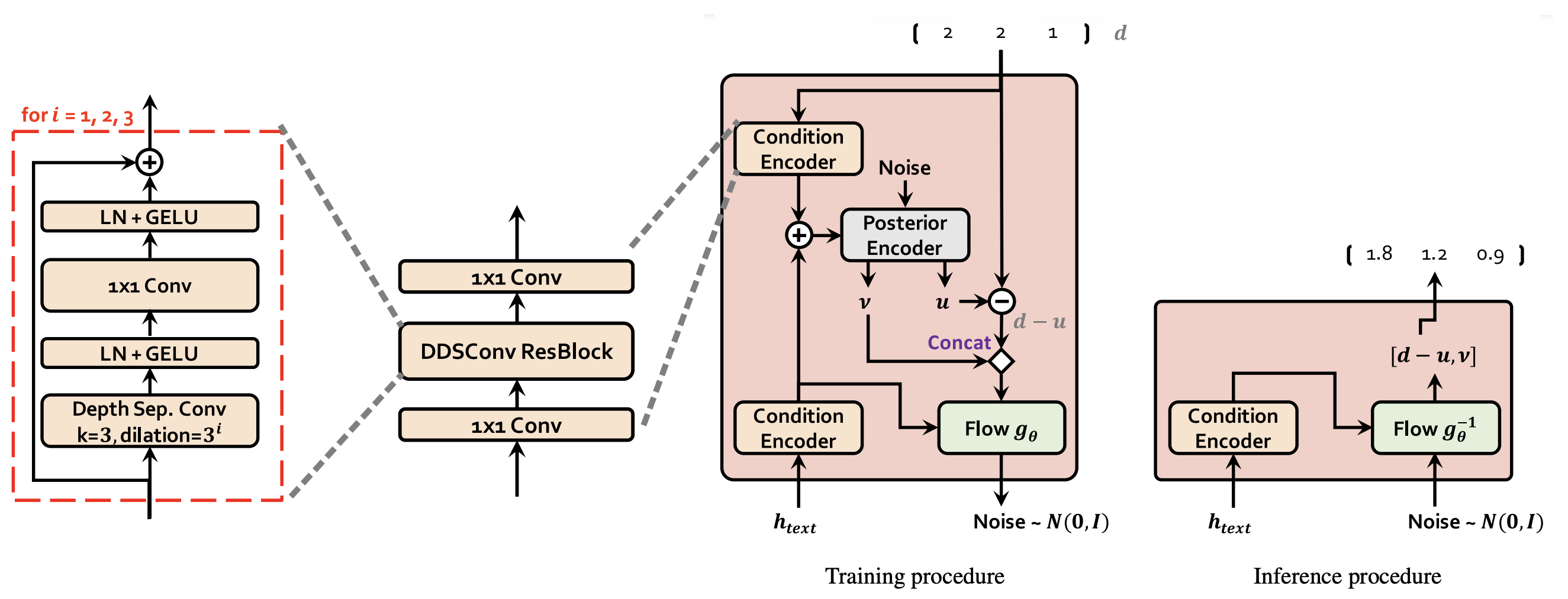
As you can see, the main building block of the stochastic duration predictor is the dilated and depth-wise separable convolutional (DDSConv ResBlock). Each convolutional layer in DDSConv blocks is followed by a layer normalization layer and $GeLU$ activation function. We choose to use dilated and depth-wise separable convolutional layers for improving parameter efficiency while maintaining large receptive field size.

For the efficient parameterization of the stochastic duration predictor, they stacked residual blocks with dilated and depth-separable convolutional layers. They also applied neural spline flows, which take the form of invertible nonlinear transformations by using monotonic rational-quadratic splines, to coupling layers. Neural spline flows improve transformation expressiveness with a similar number of parameters compared to commonly used affine coupling layers.

Note:
As you might have guessed, VITS architecture is very similar to Glow-TTS considering they both came from the same authors. VITS uses the same transformer encoder and WaveNet residual blocks as those of Glow-TTS; decoder and the multi-period discriminator as those of HiFi-GAN, except that they used different input dimension for the decoder and appended a discriminator

Loss Function

During training, VITS total loss function $\mathcal{L}_{vits}$ can be expressed as a combination of five different loss functions as shown in the following formula:

Where:

• Reconstruction Loss $\mathcal{L}_{recon}$:
  The reconstruction loss is the L1 loss between the predicted mel-spectrogram $\widehat{x}_{mel}$ and target mel-spectrogram $x_{mel}$:

• KL-Divergence Loss $\mathcal{L}_{kl}$:
  In general, KL-Divergence measures how two different distribution are matching. In this context, we are measuring the divergence loss between the posterior distribution $q_{\phi}\left( z \middle| x_{lin} \right)$ resulting from the posterior encoder, and the prior distribution $p_{\theta}\left( z \middle| c_{text},\ A \right)$ resulting from the prior encoder.

• Duration Loss $\mathcal{L}_{dur}$:
  The duration loss is the negative variational lower bound where the duration predictor vector $d$ is varitionally-quantized into two same-dimension vectors $u$ and $v$:

• Adversarial Loss $\mathcal{L}_{adv}(G)$:
  The adversarial loss is the least-squares loss between the output waveform generated by the decoder $G(z)$ and the ground truth waveform $y$:

• Feature Matching Loss $\mathcal{L}_{fm}(G)$:
  The feature matching loss is the average reconstruction loss of the discriminator $D$ hidden features of the ground truth waveform $y$ and the generated one from the decoder $D(z)$ for every layer $l$ out of $T$ total layers knowing that $N_{l}$ is the total number of features at layer $l$.

Note:
The last two loss functions heavily depend on the discriminator, which is trained interchangeably to distinguish between the generated waveform $G(z)$ and the ground truth waveform $y$ using the following loss function:

\[\mathcal{L}_{adv}(D) = \mathbb{E}_{(y,z)}\left\lbrack \left( D(y) - 1 \right)^{2} + \left( D\left( G(z) \right) \right)^{2} \right\rbrack\]

Experiments & Results

For the single-speaker experiments, they used the LJ Speech dataset which consists of $13,100$ short audio clips of a single speaker with a total length of approximately 24 hours. The audio format is 16-bit PCM with a sample rate of $22\ kHz$, and they used it without any changes. They randomly divided the dataset into a training set ($12,500$ samples), validation set ($100$ samples), and test set ($500$ samples).

Regarding audio preprocessing, they used linear spectrograms which can be obtained from raw waveforms through the Short-time Fourier transform (STFT), as input of the posterior encoder. The FFT size, window size and hop size of the transform are set to $1024$, $1024$ and $256$, respectively. They used $80$ bands mel-scale spectrograms for reconstruction loss, which is obtained by applying a mel-filterbank to linear spectrograms.

Regarding textual preprocessing, they used International Phonetic Alphabet (IPA) sequences as input to the prior encoder. They used the open-source phonemizer package to convert text sequences to IPA phoneme sequences, and the converted sequences are interspersed with a blank token following the implementation of Glow-TTS.

VITS was trained using the AdamW optimizer with $\beta_{1} = 0.8,\ \beta_{2} = 0.99$, and weight decay $\lambda = 0.01$. The learning rate decay is scheduled by a $0.9991/8$ factor in every epoch with an initial learning rate of $2 \times 10^{- 4}$. To reduce the training time, they used windowed generator training which means that they extracted segments from ground-truth waveform and latent representations with a window size of $32$ to feed to the decoder instead of feeding entire audio. VITS was trained for up to $800k$ steps.

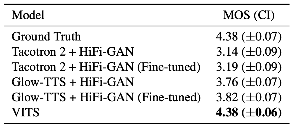
To measure the speech quality, they used crowd-sourced MOS tests where raters listened to randomly selected audio samples, and rated their naturalness on a 5 point scale from 1 to 5. Raters were allowed to evaluate each audio sample once, and audio was normalized to avoid the amplitude effect. The following table shows the MOS of VITS compared to the ground truth, Tacotron 2, and Glow-TTS where HiFi-GAN was used as a vocoder.

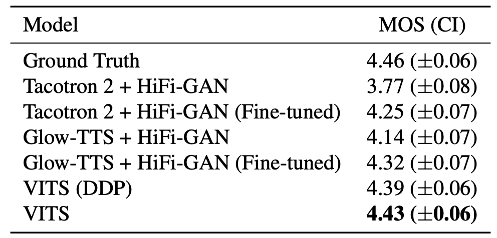
As you can see from the previous table, VITS outperforms other TTS systems and achieves a similar MOS to that of ground truth. The VITS (DDP), which employs the same deterministic duration predictor architecture used in Glow-TTS, scores the second-highest among TTS systems in the MOS evaluation.

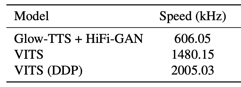
Also, they compared the synthesis speed of VITS with Glow-TTS+HiFi-GAN. The elapsed time was measured over the entire process to generate raw waveforms from phoneme sequences with $100$ sentences randomly selected from the test set. The results are shown in the following table which shows that VITS can generate up to $1480.15 \times 1000$ audio samples per second which is $\sim 3 \times$ faster than Glow-TTS+HiFi-GAN. and it takes around

Additionally, they conducted an ablation study to demonstrate the effectiveness of different components of VITS. All models in the ablation study were trained up to $300k$ steps. The results are shown in following table:

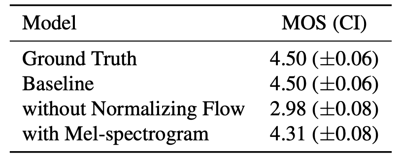
As shown, removing the normalizing flow in the prior encoder results in a 1.52 MOS decrease from the baseline. Replacing the linear-scale spectrogram for posterior input with the mel-spectrogram results in 0.19 MOS decrease.

Multi-speaker Experiments

To verify that VITS can learn multi-speaker characteristics, they trained in on VCTK dataset which consists of approximately $44,000$ short audio clips uttered by $109$ native English speakers with various accents. The total length of the audio clips is approximately $44$ hours. The audio format is 16-bit PCM with a sample rate of $44\ kHz$, and they reduced it to $22\ kHz$. They randomly split the dataset into a training set ($43,470$ samples), validation set ($100$ samples), and test set ($500$ samples).

They compared it with Tacotron 2 and Glow-TTS. For Tacotron 2, they broad-casted speaker embedding and concatenated it with the encoder output, and for Glow-TTS, they applied the global conditioning, which was originally proposed in WaveNet. For VITS, they did the following changes:

• They used global conditioning (proposed in WaveNet) in the residual blocks of the Posterior Encoder.

• They used global conditioning in the residual blocks of the normalizing flow of the BU.

• They added a linear layer that transforms speaker embedding and add it to the input latent variables $z$ before inserting it to the Decoder.

• They add a linear layer that transforms the speaker embedding and add it to the input $h_{text}$ before inserting it to the Stochastic Duration Predictor.

The evaluation method is the same as that described in the single-speaker setup. As shown in the following table, VITS achieves a higher MOS than Tacotron 2 and Glow-TTS which demonstrates that VITS learns and expresses various speech characteristics in an end-to-end manner.